Introduction

Graph theory offers an intuitive way to represent relationships between objects. As mentionned in this other post, it has numerous applications in social network theory, scheduling and routing. It can even be applied in urban planning contexts to study the structure of road networks and evaluate the effect of proposed infrastructure on traffic flows. ¹ This post, considers a similar perspective, but focuses on the structure of the graphs formed by considering partitions of a geographic unit such as neighbourhoods and how these partitions/tiles are related. The end goal is to answer the following questions:

• Are the Montreal and Quebec graphs structurally different and if so why or why not?
• What are the most central and peripheral neighbourhoods of each city?
• Can we use graph theory to identify groups of related neighbourhoods?
• Can we use graph theory to study population density?

Basic formalism and setup

We consider a graph \(G=(V,E)\) composed of \(|V|=n\) nodes and \(|E|=m\) edges between them. In our case, the nodes \(V\) are taken as some representative point within a given tile (for instance the centroid of a neighbourhood). There is an edge \((u,v) \in E \subset V \times V\) if the tile \(u\) touches the tile \(v\) (more technical details on this later). For each edge \(e \in E\), we can associate a given weight \(w(e) \in \mathbb{R}_+\). If \(w(e)=1,\forall e \in E\), we say the graph is unweighted.

We let \(d_G(i)\) denote the degree of a node \(i \in V\) in graph \(G\), which represents the number of nodes adjacent to \(i\). A clique with \(k\) nodes in \(G\) is a subgraph \(K_k = (V',E') \subset G\) such that \(|V'|=k\) and \(d_{K_k}(u) = k-1, \forall u \in V'\).

Given a distance function \(d: V\times V \rightarrow \mathbb{R}_+\), the node eccentricitity of node \(v\) is defined as the longest distance from \(v\) to any other node: \(\epsilon(v) = \max_{u} d(u,v)\). We define the graph diameter \(D_G\) and radius \(r_G\) as the maximum and minimum eccentricty respectively: \(D_G = \max_{u \in V} \epsilon(u)\) and \(r_G = \min_{u \in V} \epsilon(u)\).

If nodes \(u\) and \(v\) are associated with a longitude and latitude, then we can consider a weighted graph and \(d(u,v)\) can represent as-the-crow-flies distance between \(u\) and \(v\). In an unweighted scenario, \(d(u,v)\) can simply represent the minimum number of edges required to reach \(v\) from \(u\).

In the rest of this post, we will consider 2 different types of partitions. The first is the tiling formed by the neighbourhoods composing a city. This is a natural partition of the space and has intuitive appel. However, it can only be applied to cities. Moreover, since neighbourhoods bear a sociological dimension, they may have unwieldy shapes with very different population sizes.

The second approach is based on tiles formed by dissemination areas (DAs). This offers an interesting perpective since DAs are used by Statistics Canada as a granular sociodemogrphic unit whose population is supposed to be composed of 400 to 700 individuals. Hence, DA size is a decreasing function of population density and the strucutre of the associated graph reveals important caracteristics about the region.

A quick glance at Montreal and Quebec graphs at the DA level

We first consider the graphs formed by the DAs partitioning Quebec and Montreal:

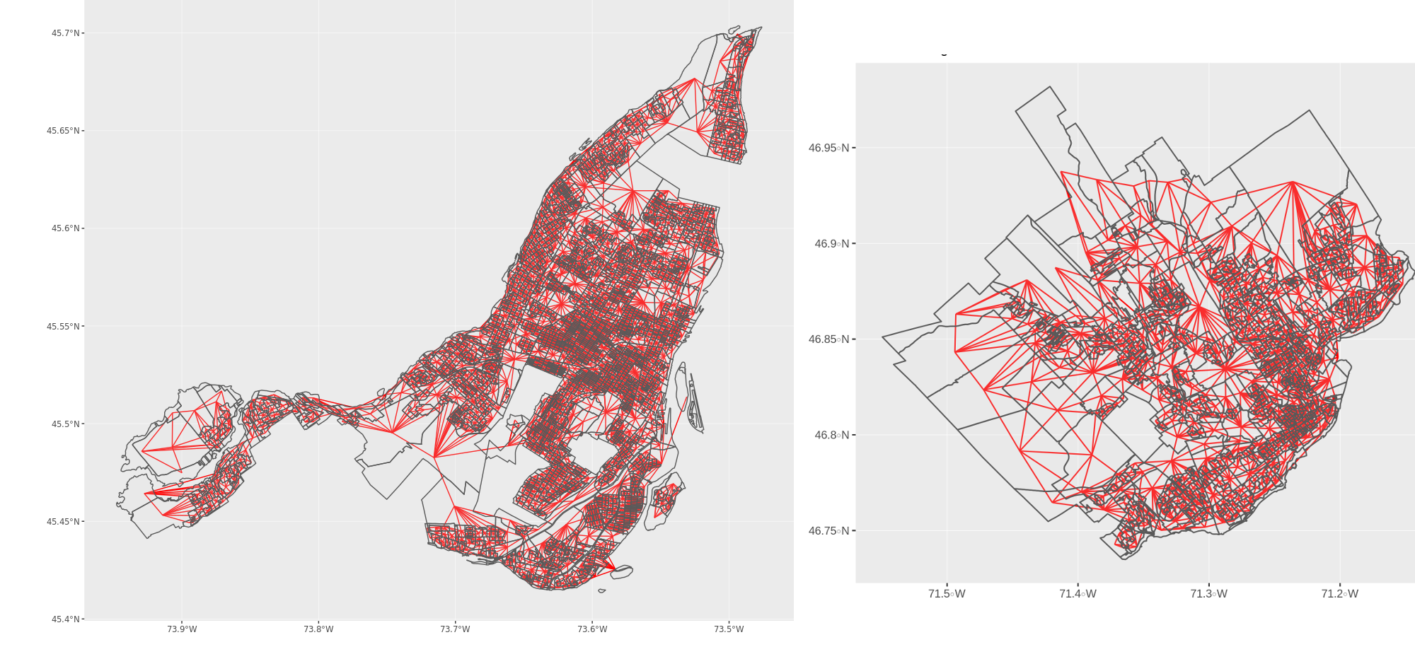
Graph of Montreal and Quebec - by DA

We immediately notice there are much more nodes and edges in the Montreal graph since DAs are assumed to have similar population and Montreal is 2 to 3 times more populated than Quebec City. It is hard to make out solely by looking at those pictures, but there also seems to be a higher proportion of large DAs with high degree in Quebec.

Exploring graph metrics

It is possible to refine our understanding of the city structures by considering some simple graph theoretic metrics. We start by comparing the degree distribution of both cities and the entire Quebec province graph.

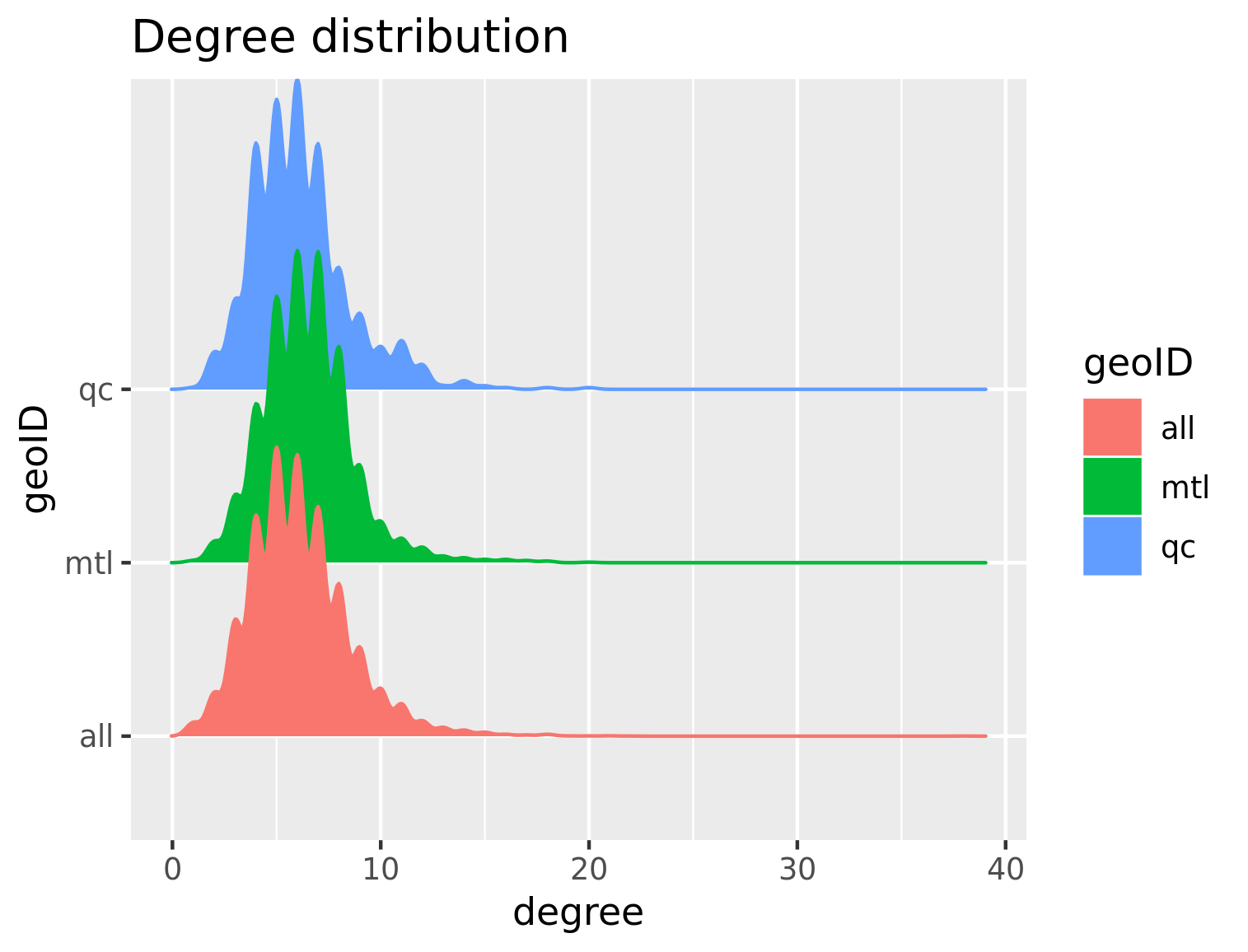
Degree distribution - Montreal and Quebec - by DA

Perhaps surprisingly, the 3 distribution are qualitatively similar. ² The very rare nodes with a huge degree correspond to the sparse DAs mentionned previously.

We next consider the eccentricity distribution with the unweighted graphs to highlight differences in graph structure that are independent of physical distances. Even without factoring in physical distance, we notice stark differences. The fact that all eccentricities are similar for Quebec is an artefact of the circular shape of the city’s administrative boundaries. On the other hand, the more elongated shape of Montreal means that there is more variability in the eccentricities and that on average, the eccentricity is larger. The variance is even more pronounced for the entire province graph.

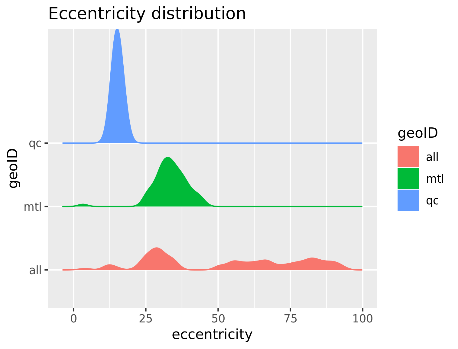
Eccentricity distribution - Montreal and Quebec - by DA

What are the most peripheral and central neighbourhoods?

Considering eccentricities is interesting in an urban planning context. It allows us to identify nodes that are central by considering those achieving the radius of the graph. On the other hand, nodes achiving the diameter are more peripheral. To get a better intuition, we consider neighbourhoods rather than DAs in the following section.

Central neighbourhoods

For Quebec City, the most central neighbourhood is Neufchâtel-Est/Lebourgneuf (in the center of the figure). It achieves the radius both for the weighted and unweigthed cases. Starting from that neighbourhood centroid, it is possible to can reach any neighbourhood in at most 14 km ³. The neighbourhood furthest from Neufchâtel is Cap-Rouge (bottom left).

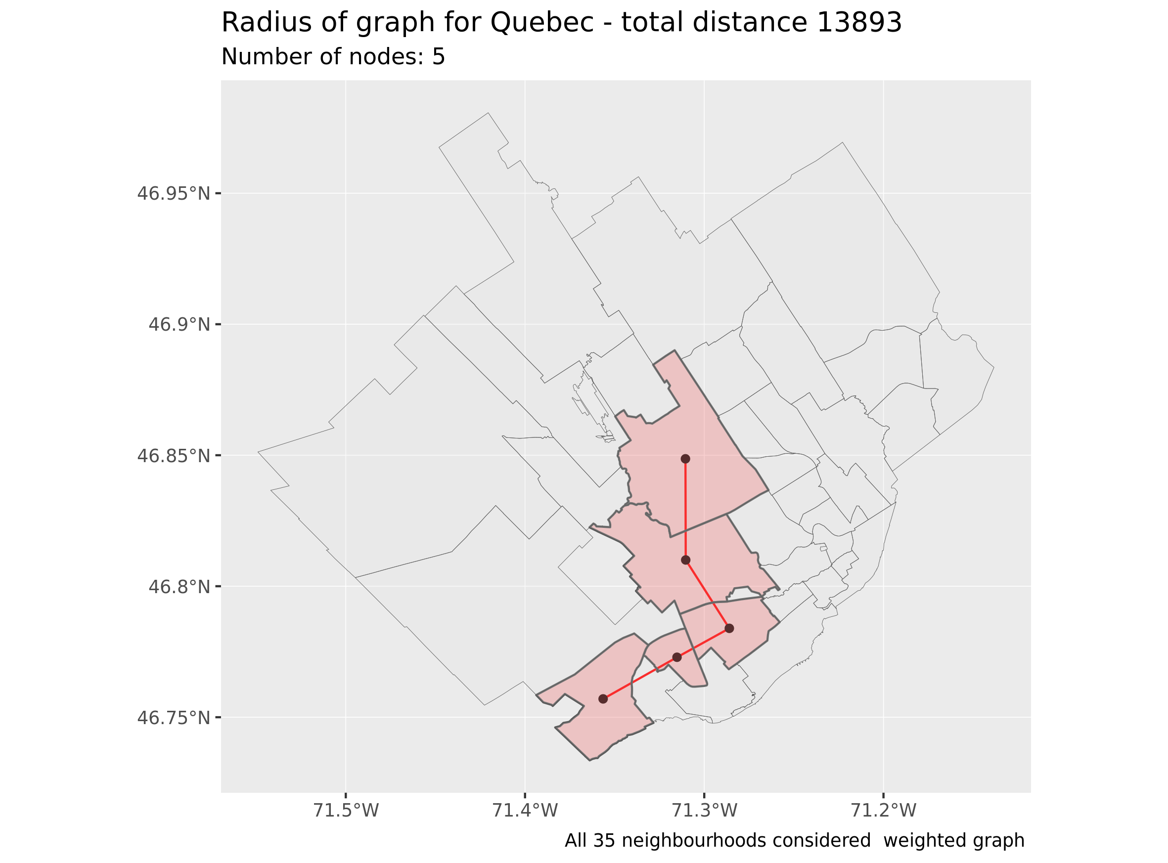
Quebec radius - weighted graph - as-the-crow-flies

For Montreal, the most “central” neighbourhood in terms of eccentricity turns out to be Ahuntsic (in the center of the island) and the furthest neighbourhood from Ahuntsic is the West-Island. The radius is more than 5 km larger for Montreal than for Quebec. This might seem slightly counterintuitive given Quebec actually covers a larger area, but is once again a consequence of the difference in city shapes. To put these numbers in perspective, the radius of the graph obtained by considering the DAs above the \(55^{th}\) parallel is equal to more than 808 km. This is to be expected since those DAs as well as the distance between them are huge.

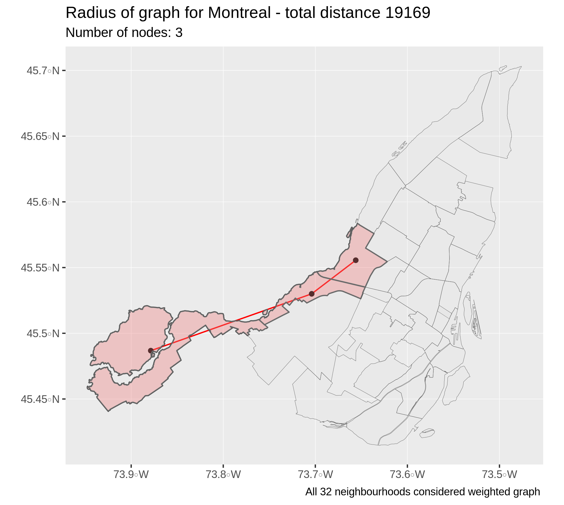
Montreal radius - weighted graph - as-the-crow-flies

Peripheral neighbourhoods

Now that we’ve identified the central neighbourhoods as those with minimal eccentricity, we can consider peripheral neighbourhoods as those achieving the graph diameter (with maximal eccentricity).

In the case of Quebec City, the most peripheral neighbourhoods are Chutes-Montmorency (right) and Val-Bélair (left). Going from one neighbourhood to the next requires travelling more than 24 km and passing through 8 differents neighbourhoods.

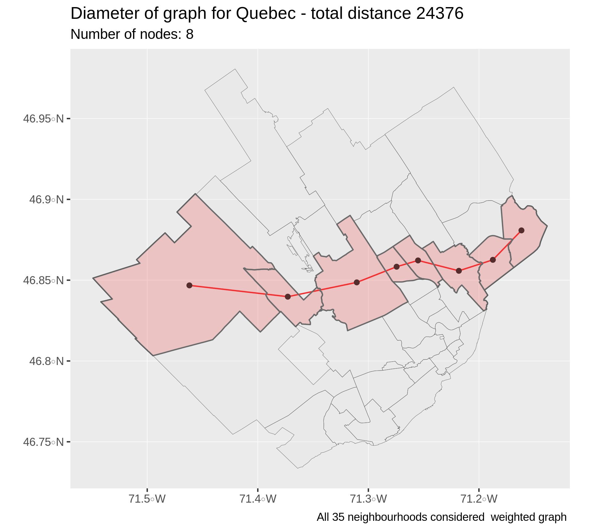
Quebec diameter - weighted graph - as-the-crow-flies

For Montreal, as can be expected the most peripheral neighbourhoods are at the extreme east and west of the island, which jibes well with the traditional linguistic divide of the city. This also somewhat matches the path of Boulevard Gouin, which is the longest street of the city if I recall correctly.

Compared with Quebec City, the diameter is over 12 km longer, but passes through 2 fewer neighbourhoods. This can be explained by the very irregular dimensions of the neighbourhoods as well as the rather elongated shape of Montreal.

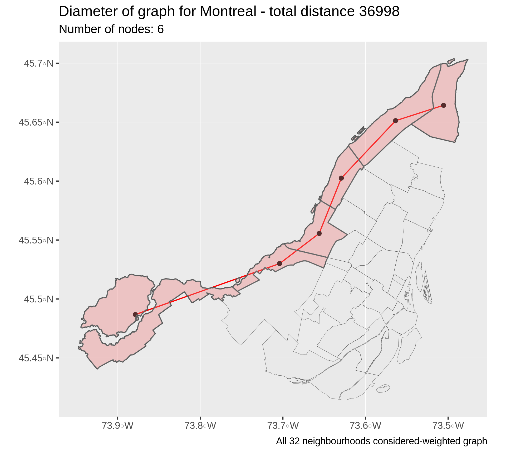
Montreal diameter - weighted graph - as-the-crow-flies

Cliques

We next study the cliques of the city graphs. Cliques represent maximally connected subsets of nodes that are linked to every other node in that set. For the city graphs we consider, cliques represent sets of DAs or neighbourhoods that all share common boundaries and are therefore close to one another. Because of this proximity, they may share common histories, sociodemographic profiles and therefore represent natural clusters.

DA level

The following figure, taken at the DA level, reveals that once again, the distribution seem qualitatively similar for both cities. For both cities, the majority of cliques are of size 3, but there are some of size 4 and even 5 ⁴. The plot obscurs the fact that there are much more large cliques in Montreal: there are 4 cliques of size 5 in Quebec and 15 cliques of size 5 in Montreal.

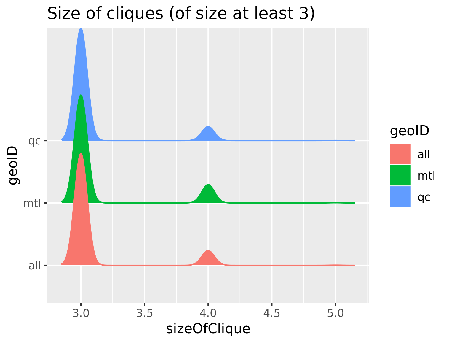
Clique distribution

For illustration purposes, here are the maximal cliques for Quebec City as well as a zoomed version of the red clique in Beauport, Quebec.

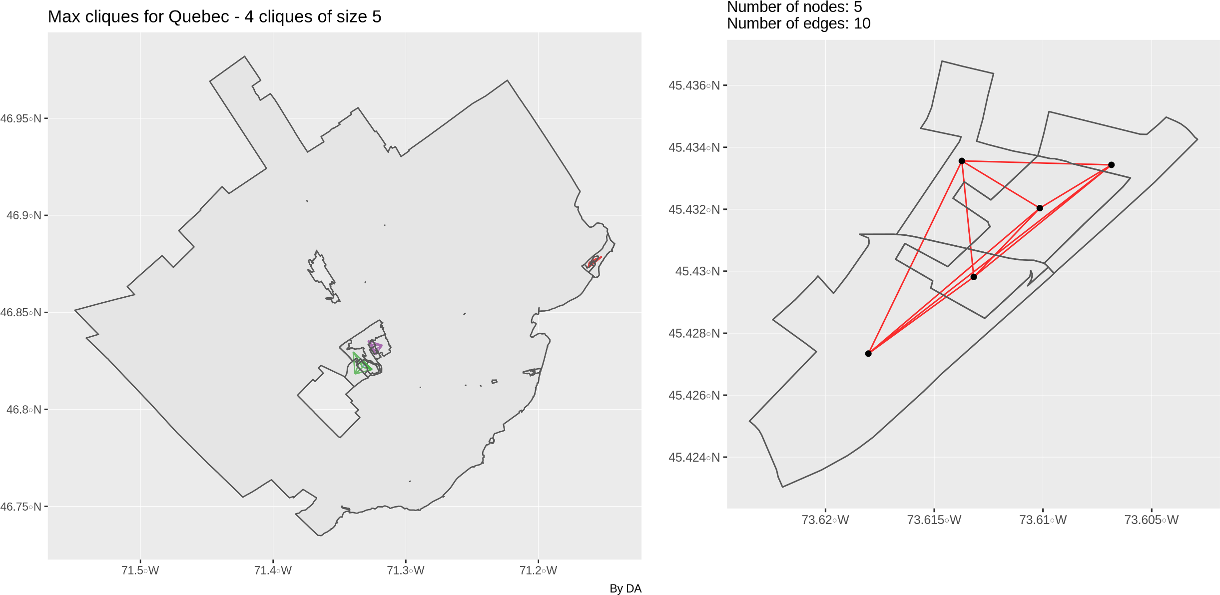
Maximal cliques of size 5 in Quebec

Neighbourhood level

At the neighbourhood level, maximal cliques reveal interesting information. The clique formed of Saint-Henri, Ville-Emard, Pointe-Saint-Charles and Verdun forms a natural sociodemographic cluster, as does Saint-Michel, Villeray, Petite-Patrie and Rosemont. It is tempting to suggest that neighbourhoods such as Rosemont that belong to different maximal cliques may also be seen as natural bridges between communities, but this might be pushing the interpretation a bit far. Indeed, cliques are only derived from geographical contiguity data. Le plateau and Rosemont may be considered more or less homogeneous in terms of demography, but they are surely different from Hochelaga and Centre-Sud.

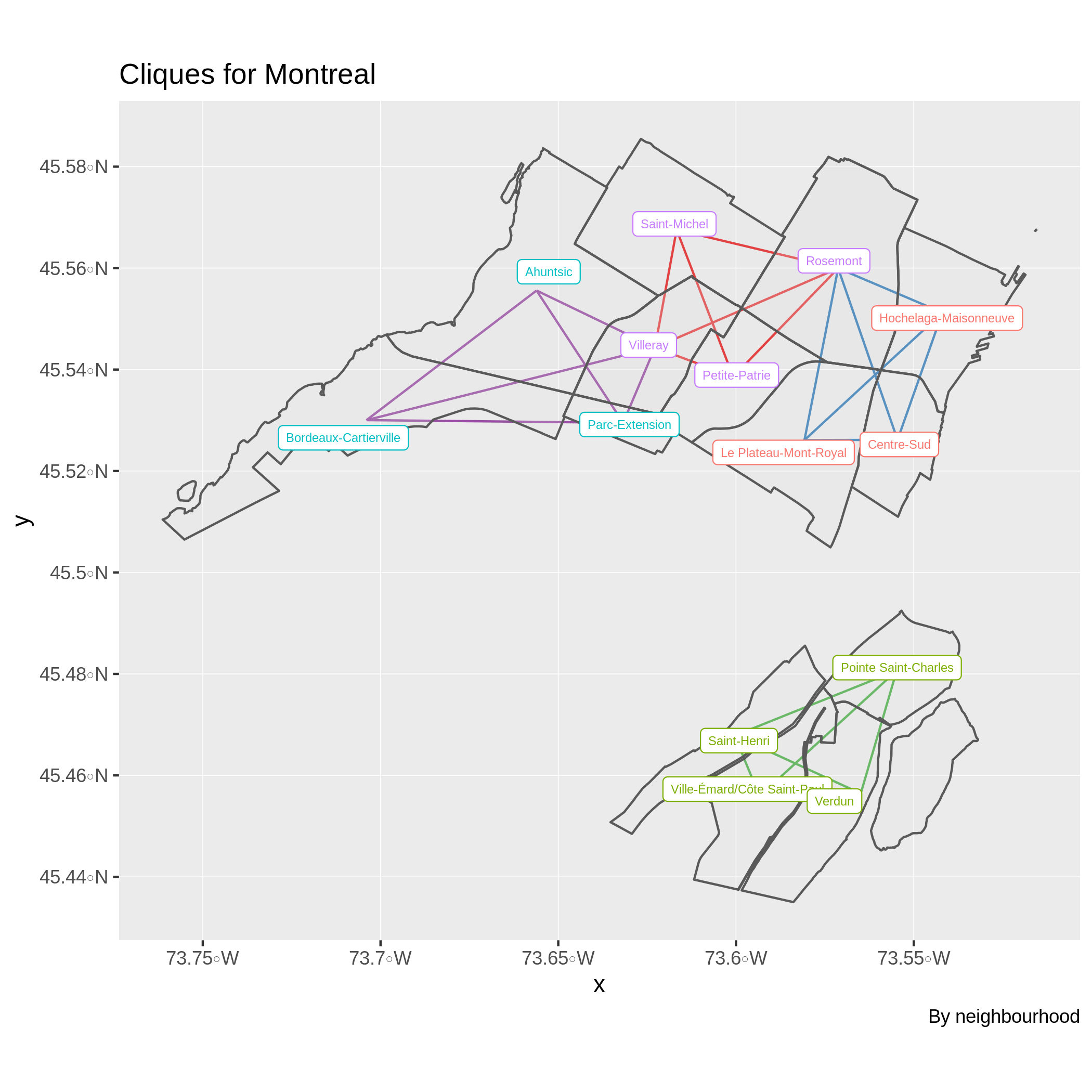
Neighbourhood Cliques - Montreal

In the case of Quebec City, the neighbourhoods Vieux-Quebec, Saint-Roch, Montcalm and Saint-Jean-Baptiste all hold foremost importance in the history of the city. See this post for more details. It is also unsurprising that Saint-Jean-Baptiste appears in 2 different maximal cliques due to its central position.

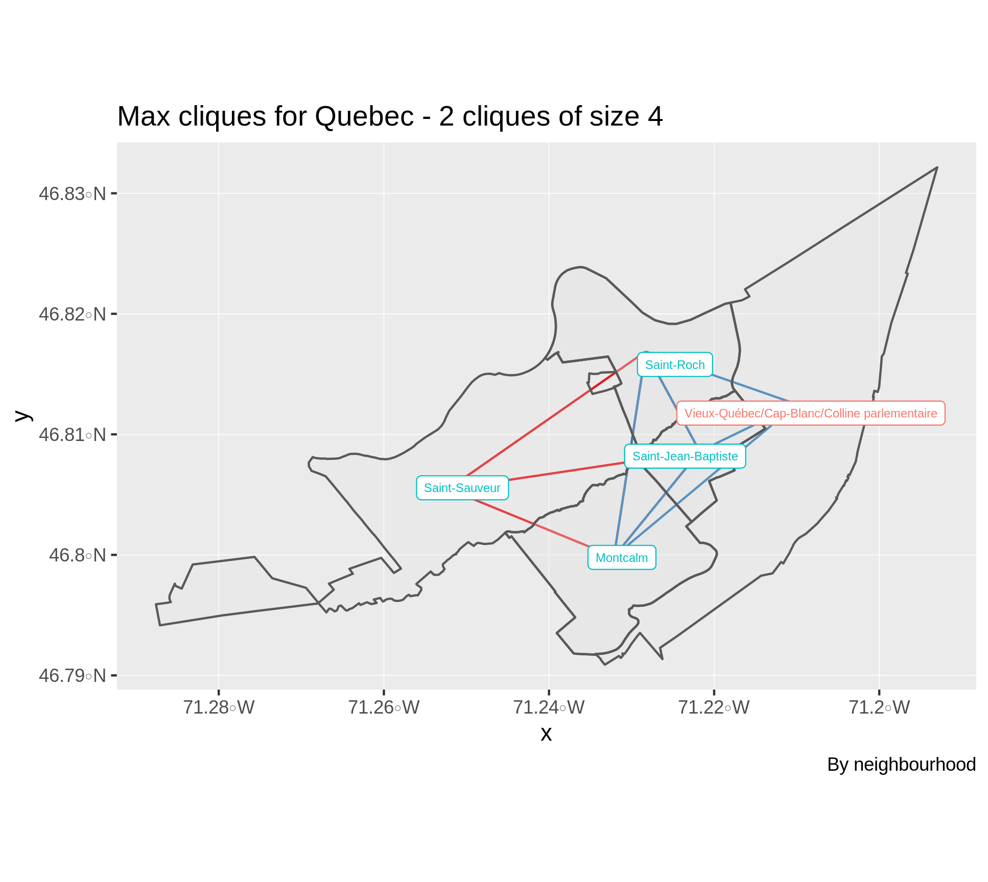
Neighbourhood Cliques - Quebec

Graph diameter and population density

Perhaps surprisingly, comparing the graph diameters of the weighted (edge weights equal to as-the-crow-flies distance) and unweighted (edge weights all equal to 1) graphs when the nodes represent DA centroids reveals interesting population density patterns.

In the case of Montreal, the following figure shows that considering a weighted or an unweighted graph leads to paths of similar total distance passing through roughly the same DAs.

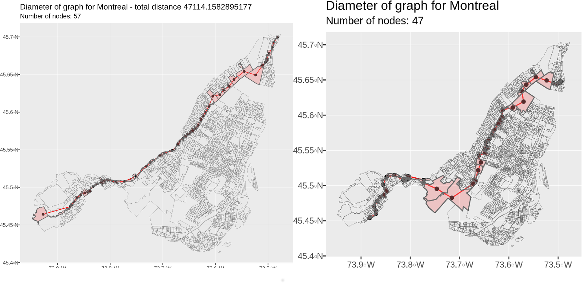
Montreal diameter - DAs - weighted vs unweighted graph

This picture is rather different for Quebec. Indeed, the maximum shortest path attaining the graph diameter for the unweighted graph manages to pass through a series of large sparsely populated DAs. This path is composed of 12 fewer edges than the path achieving the diameter for the weighted graph. This is a larger difference than the 10 fewer edges required in the case of Montreal. Indeed, there is a 38% edge reduction in the case of Quebec City while this value is only 18% for Montreal.

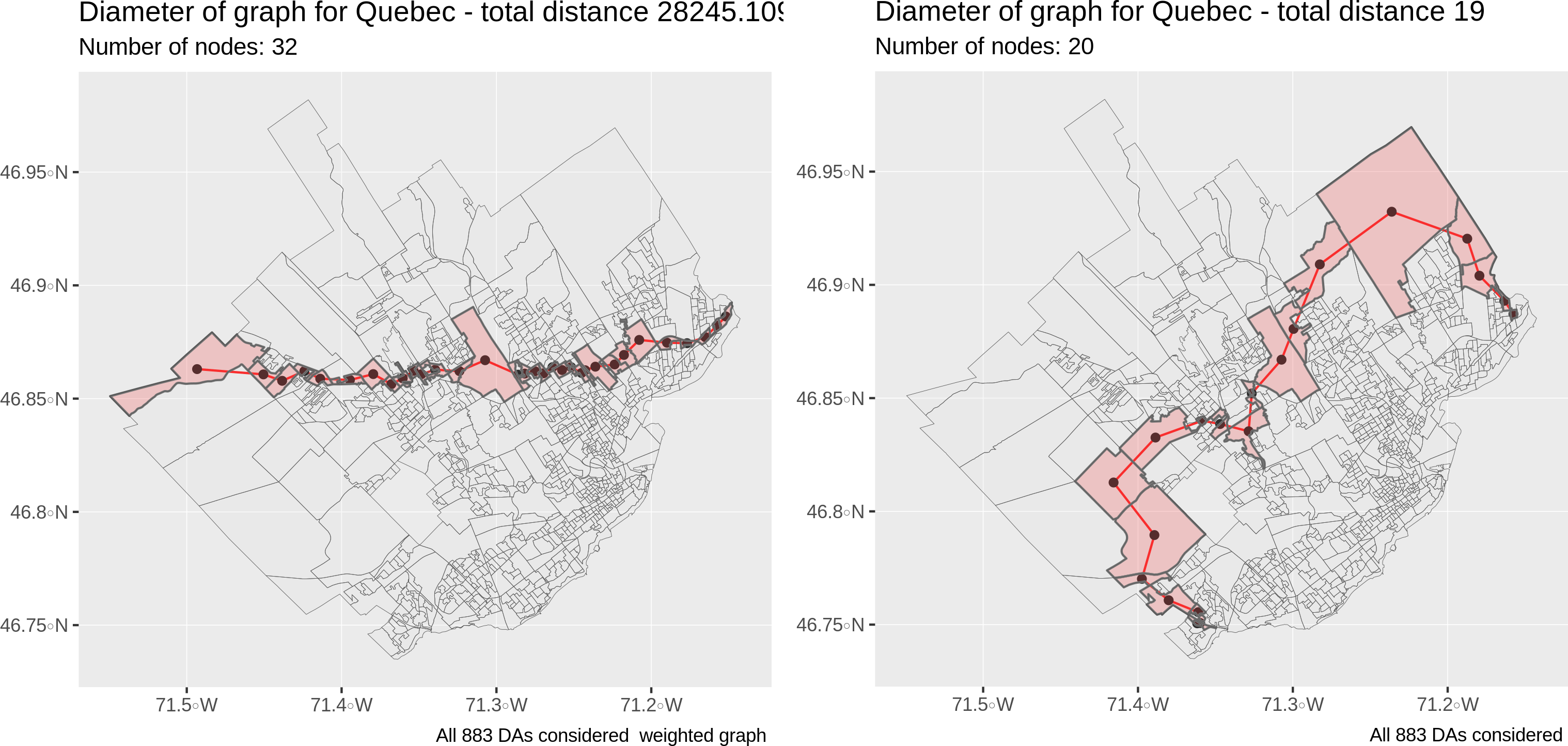
Quebec diameter - DAs - weighted graph - as-the-crow-flies

The large difference in graph diameters for weighted and unweighted graph can be partly linked to the variability in population densities. If the population density is uniform over a given region and DAs also have regular shapes, then the graph will be close to a regular grid/lattice. In this case, nodes achieving the graph diameter will be the same in the weighted and unweigthed case. This hypothesis is corroborated by the following graphs, which were created by considering a regular lattice over the city of Montreal.

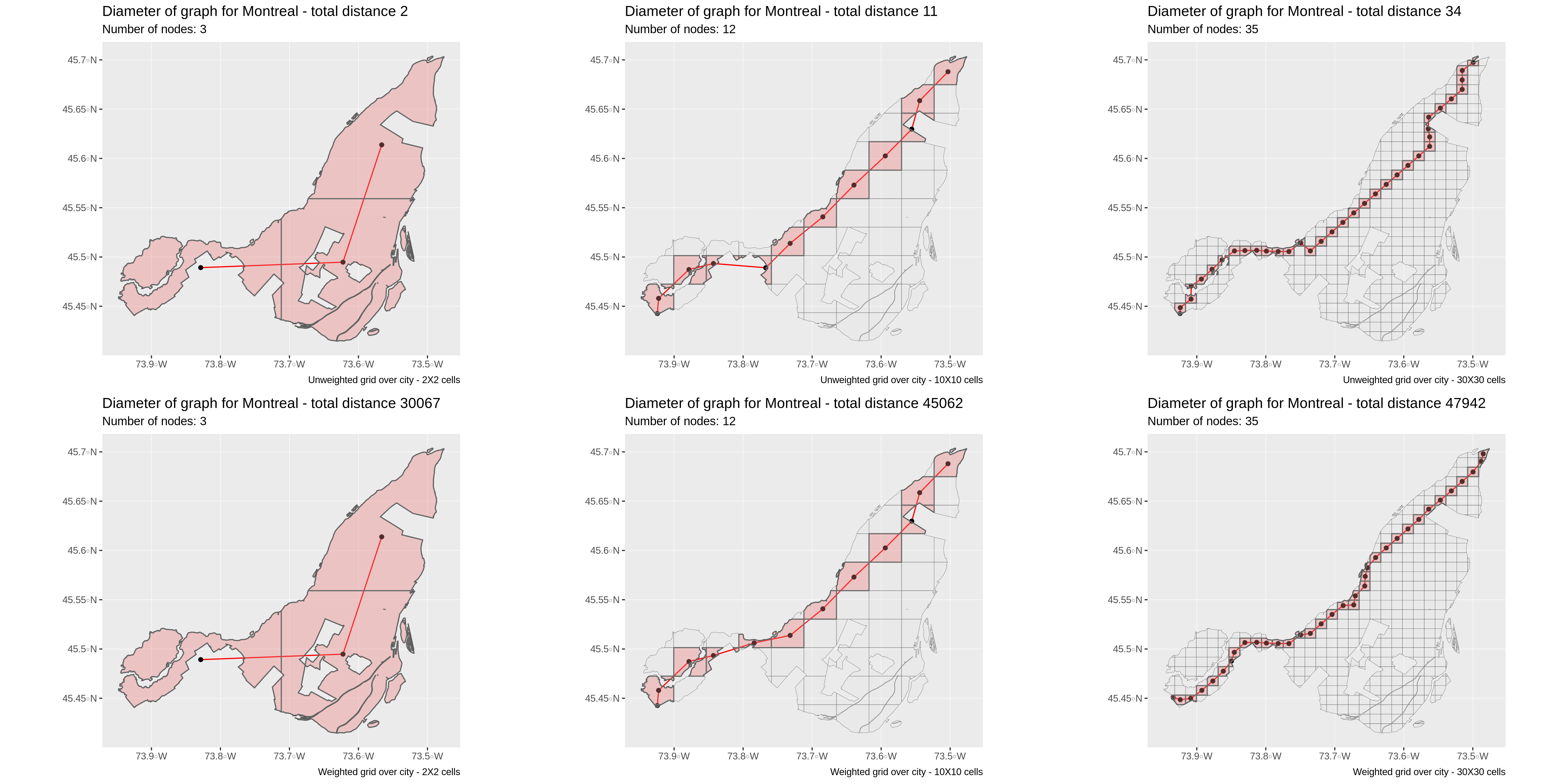
Montreal diameter on regular grid graph - weighted vs unweighted graph

This is also true in the case of Quebec City. Although the path achieving the diameter in the \(30 \times 30\) lattice unweighted graph (top right) is very different from the one in the same \(30 \times 30\) weighted graph (bottom right), the path in the weighted case also achieves the diameter of 31 edges and 30 nodes. The apparent contradiction is an artefact of the circular shape of the city and the fact that there are multiple paths achieving the diameter. In any case, both weighted and unweighted diameters have the same number of edges, which is not observed empirically.

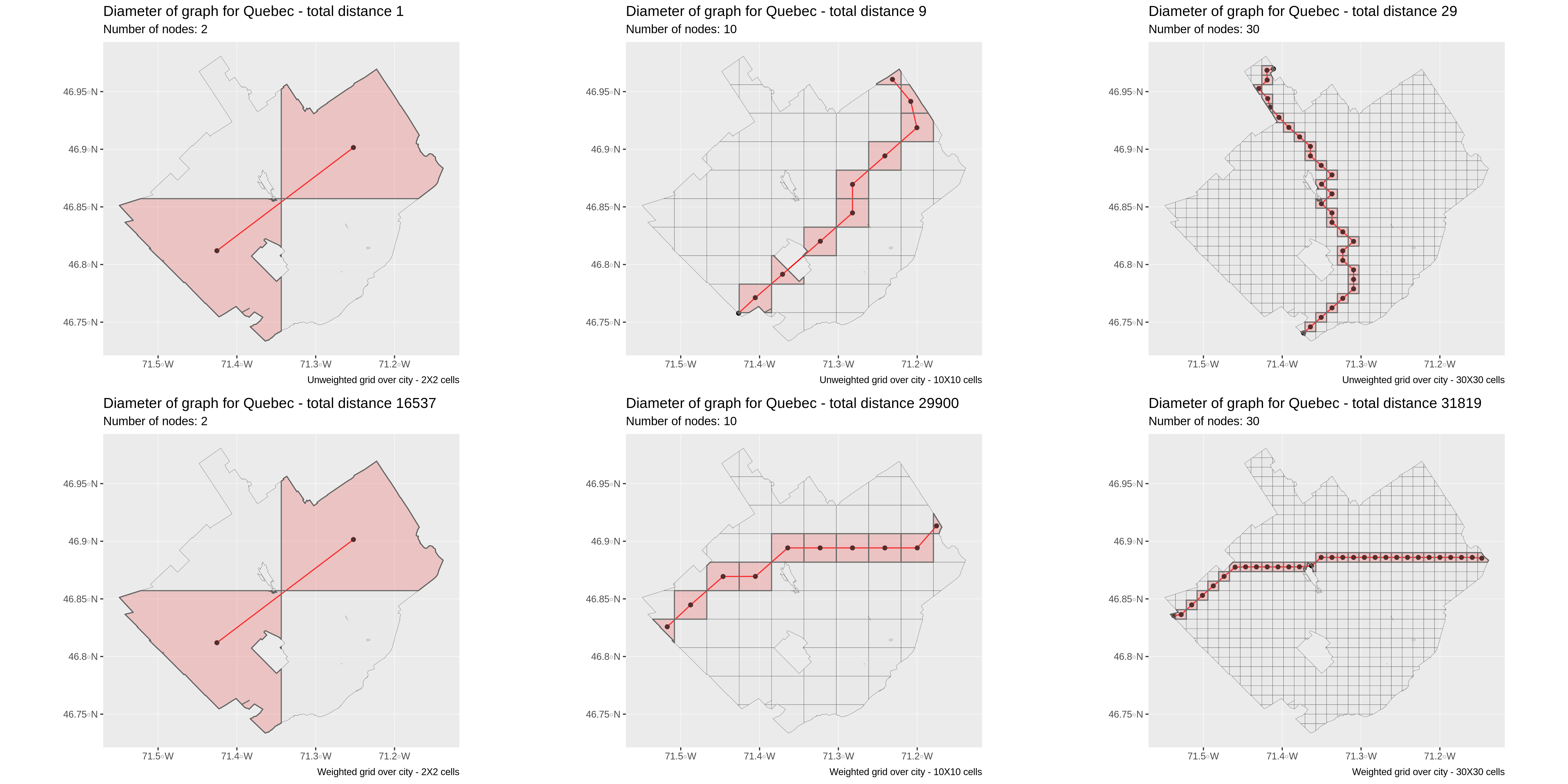
Quebec diameter on regular grid graph - weighted vs unweighted graph

Although this simple analysis makes multiple assumptions on DA shapes and sizes that are not always observed in practice, it remains interesting. It also confirmed prior observations that both cities have very different shapes.

Conclusion

We’ve just shown that is it possible to use graph theory together with basic geospatial data to analyze multiple aspects of a city such as:

• Population density
• Shape
• Centrality/peripherality of neighbourhoods
• Physical proximity of neighbourhoods

More specifically, we’ve seen that although there exists large sparsely populated regions in Montreal, the island is much denser than Quebec City. We’ve also highlighted the fundamentally different shapes of both cities. Montreal has a smaller area and is elongated, while Quebec ic circular.

Appendix

Technical details on the graph creation

If you’ve ever heard of the famous four color and Kuratowski theorems, then you know that finding a clique of size 5 in a planar graph is impossible. The confusion stems from technical details related to the way the city graphs are constructed. More specifically, the source of the problem is the way the sf package in R defines “adjacency”. For instance, in the sample clique from Beauport, Quebec in red above, many DAs only touch at a single point.

The figures below illustrates the difference in the graphs obtained by considering sf::st_touches on the left and sf::st_intersects on the right. Note that it is also possible to use spdedp::nb2poly with “queen” or “rook” arguments to produce similar results. The analysis above was produced with sf::st_intersects, which seemed to produce more reliable results.

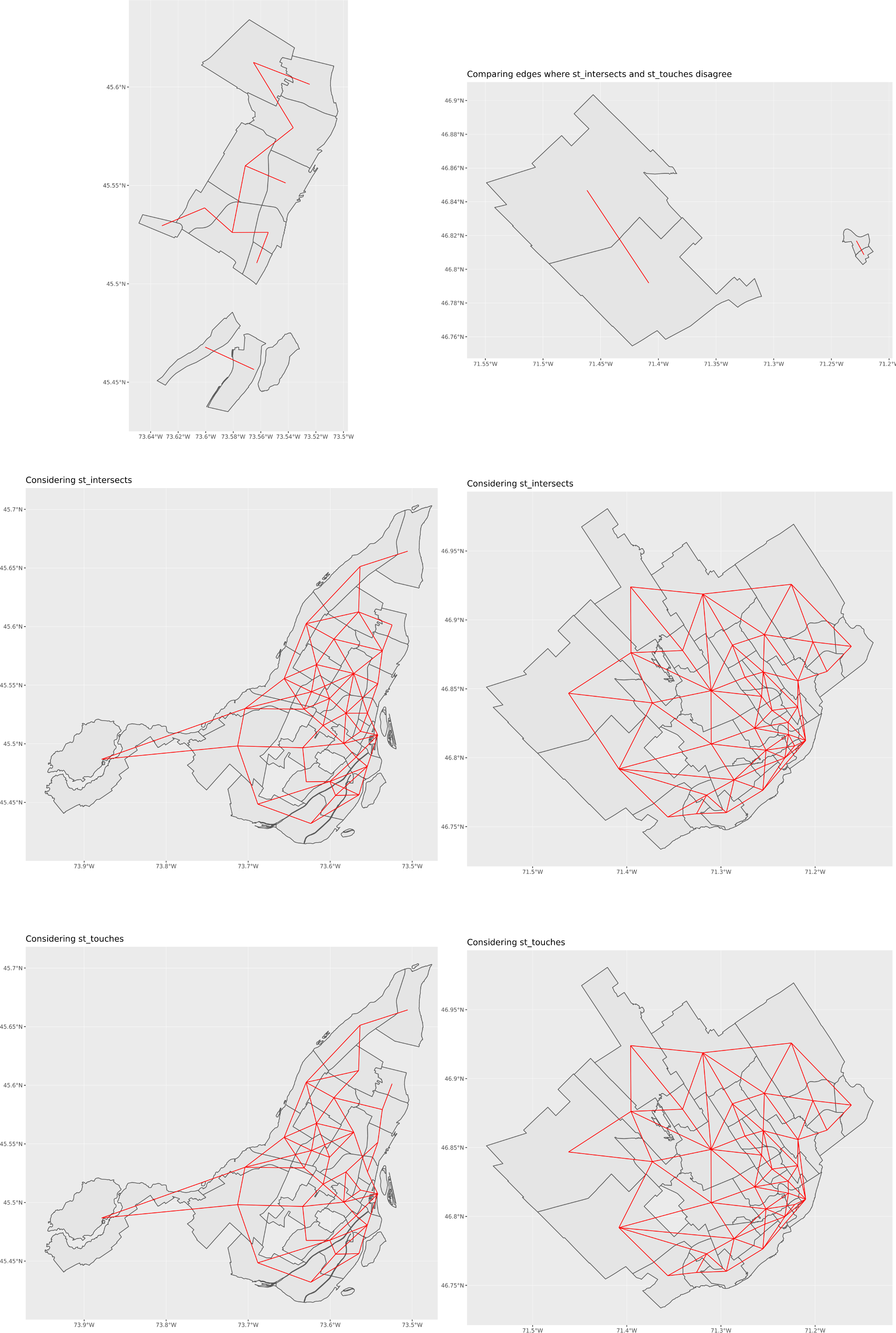
Spatial predicates comparison - Montreal (left) - Quebec (right)