
Notes on clustering
Introduction
Clustering algorithms have various important applications, namely in exploratory data exploration, political districting, image compression, etc.
In essence, we seek an assignment of \(n\) objects with a set of \(p\) attributes/features to \(k=|C|\) groups \(C=\{C_1,\cdots,C_{k}\}\) in order to minimize some total distance metric and create homogeneous categories. The number of groups is usually fixed in most algorithms, such as the popular \(k\)-means, but could also be considered as a variable in \(\{1, \cdots, n\}\). Clustering problems are hard to solve exactly. The minimum diameter clustering problem in the plane was already recognized as NP-Hard by Garey and Johnson.
Because of their ubiquity and the challenge of solving them numerically, algorithms have attracted a considerable amount of research from different disciplines including statistics, social network theory, graph theory and combinatorial optimization. Due to their different motivations, these domains all provide different and complementary perspectives on the problem.
This document gives a quick overview of various distance metrics used in different disciplines in order to define clusters as homogeneous or related groups of points. These notes are only used to illustrate certain concetps and are in no way meant to be an exhaustive.
Notation and basic identities
Before explaining the various metrics and methods used for clustering, it is useful to define some graph theory terms which will used throughout the document. A graph essentially codifies the relationship between a set of points. Nodes/vertices represent points or observations and edges represent relationships between them. Graphs can be directed or undirected. In the former case, the relationship between nodes \(v_i\) and \(v_j\) is not the same as the one between \(v_j\) and \(v_i\) and in the latter this relationship is symmetric.
Unweighted graphs have edges that have a binary \(\{0,1\}\) weight indicating presence of absence. On the other hand, weighted graphs may have real weights which can namely indicate dissimilarity.
A graph \(G=(V,E)\) is composed of \(|V|=n\) nodes and \(|E|=m\) edges between them. If \(G\) is undirected, then the orientation of edges is irrelevant and \((i,j)\) and \((j,i)\) represent the same pair. This is not be the case if \(G\) is directed and in this case we may refer to edges as arcs. Each node has degree \(d_i \in \mathbb{Z}_+\).
These notes only consider simple graphs, which are graphs with at most 1 edge between pairs of nodes. However, it is also possible to consider multigraphs where the end nodes and arc orientation are no longer sufficient to uniquely identify an edge/arc.
An undirected simple graph without self-loops of the form \((v_i,v_i)\) such that \(m = {n \choose 2} = \frac{(n-1)n}{2} = \sum_{i \in V} \frac{(n-1)}{2} = \sum_{i \in V} \frac{d_i}{2}\) has the maximum number of edges. We then write \(G=K_n\) indicating that \(G\) is the complete graph on \(n\) vertices. In this case , we also say that the graph is \((n-1)\) regular since the degree of all nodes is \(n-1\).
For an unweighted graph, \(A \in \mathbb{N}^{n\times n}\) represents the adjacency matrix where \(A_{ij}\) represents the number of edges between \(i\) and \(j\). For graphs without self loops and multiple edges, \(A_{ii}=0,\forall i\) and \(A_{ij} \in \{0,1\}\) if the edge exists and 0 otherwise. We have \(A_{ij} \in \mathbb{R}\) in the case of weighted graphs and \(A=A^{\top}\) if \(G\) is undirected.
Since each edge contributes 1 to the degree of exactly 2 nodes for simple graphs, we have \(\sum_{i \in V} d_i = 2m\). We also have \(d_i = \sum_{j \in V} A_{ij}\) and hence \(\sum_{i \in V} \sum_{j \in V} A_{ij} = \sum_{i \in V} d_i = 2m\).
An induced subgraph on a subset of nodes \(V_k= \{ v_{i_n},\cdots, v_{i_k} \}\) is a subgraph \(G_k = (V_k,E_k)\) such that \(E_k=\{(v_i,v_j) \in E: v_i,v_j \in V_k\}\) is composed only of the edges in \(E\) between nodes in \(V_k\).
A connected component is a subset of nodes such that there exists a path from any node to any other. For a directed graph, we may consider a strongly connected component if arc orientation is important.
Finaly, we let \(N_i=\{ v_j \in V : (v_j,v_i) \in E\}\) represent the neighbourhood of vertex \(v_i\) and it follows that \(d_i = |N_i|\).
Simple toy example
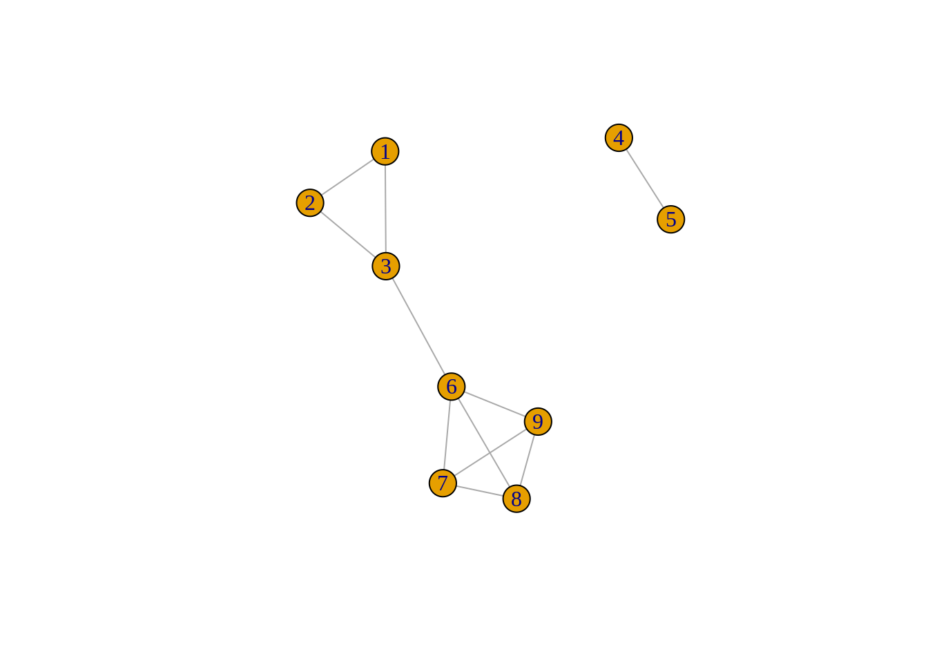
To gain intuition on the various metrics, we will consider the following simple undirected and unweighted graph composed of 9 nodes grouped into 2 disconnected components with 11 edges:
Graph theory - metrics
Social network theory is a relatively new discipline. In contrast, the problem of graph partitioning has held an important place in graph theory since many decades. As its name indicates, this problem seeks to partition nodes based on various properties and structures of the graph. This can namely be carried out by removing edges to disconnect certain portions of the graph. Recursively applying this procedure can then lead to any desired number of clusters.
Assuming that similar groups of nodes are densely connected together, it makes intuitive sense to find a subset of edges such that the removal disconnects the graph into disjoint densely connected partitions. It also makes sense to consider such sets that are in some sense minimal. This is the idea behind the following two algorithms.
Minimum cut
The minimum cut problem seeks a partition \(\{S,\bar{S} \}\) such that the weight of edges crossing from \(S\) to \(\bar{S}\) is minimized :
\[ \min_{S \subseteq V} E(S,\bar{S}) \]
where \(E(S,\bar{S})=\sum_{i \in S} \sum_{j \in \bar{S}} A_{ij}\) represents the weight of edges in the cut and \(A_{ij}\) is the \(i,j^{th}\) entry of the adjacency matrix.
This problem is easy to solve. The celebrated max-flow min cut theorem states that both the min cut and the max flow problems have the same optimal objective value. Indeed, the two problems are dual to each other and they can be solved efficiently with linear programming or other more specialized algorithms.
However, solving such a problem often leads to very poor quality solutions that often consists in isolating a single node from the rest of the graph by removing few edges. In fact for the simple toy graph used above, the graph is already disconnected and so no edges need to be removed. In general, removing \(k\) edges is sufficient if the graph is \(k\)-connected.
Sparsest cut
In order to obtain a better partition, we consider the following problem:
\[ \sigma(G) = \min_{S \subseteq V} \frac{E(S,\bar{S})}{|S||\bar{S}|} \]
minimizing this value favours partitions \(\{ S,\bar{S} \}\) with few edges between them (low \(E(S,\bar{S})\)) and balanced partitions. Indeed, \(|S||\bar{S}|\) is maximized when \(|S|=|\bar{S}|\) and \(|S| \in \{ \lceil \frac{n}{2} \rceil , \lfloor \frac{n}{2} \rfloor\}\).
Contrary to the min cut problem, this problem is difficult (NP-Hard). However, there exists approximations based on spectral graph theory. It is namely possible to derive bounds of the form:
\[ q \lambda_2 \leq \sigma(G) \leq Q \sqrt{\lambda_2}\]
for constants \(q\) and \(Q\) and \(\lambda_2\) is the second eigenvalue of \(L'\), the normalized Laplacian matrix (more details below).
Essentially, deriving the 1st inequality comes from the fact that finding the 2nd eigenvalue can be formulated as the following problem:
\[ \lambda_2 = \min_{ x \in \mathbb{R}^n \setminus \{ 0,1\} } \frac{ \sum_{u,v \in E} |x_u - x_v|^2}{ \sum_{u,v \in V^2} |x_u-x_v|^2 } \]
while finding the sparsest cut is equivalent to solving:
\[ \sigma(G) = \min_{x \in \{0,1\}^n \setminus \{ 0,1\} } \frac{ \sum_{u,v \in E} |x_u - x_v|^2}{ \sum_{u,v \in V^2} |x_u-x_v|^2} \]
it follows that the the first problem is a relaxation (lower bound) of the true sparsest cut.2
Spectral clustering algorithm are deeply connected with properties of the Laplacian matrix of the graph. The Laplacian matrix is defined as \(L=D-A\), where \(D=diag(d_1,\cdots,d_n)\) is the matrix with the degrees of the vertices on the diagonal. The normalized Laplacian is given by \(L'= D^{-\frac{1}{2}}L D^{-\frac{1}{2}} = I - D^{-\frac{1}{2}} A D^{-\frac{1}{2}}\).
We can show that \(L\) and \(L'\) are semidefinite positive (\(x^{\top}Lx \geq 0, \forall x)\) which is equivalent to having all eigenvalues greater or equal to \(0\). In fact, we can see that \(\mathbf{1} \in \mathbb{R}^n\) and \(D^{\frac{1}{2}} \mathbf{1}\) are respectively eigenvectors of \(L\) and \(L'\) with eigenvalue \(0\) since \(d_i - \sum_{j: (i,j) \in E} A_{ij} = 0, \forall i\) and \(L\mathbf{1} = 0 \cdot \mathbf{1}\) implies that \(L'D^{\frac{1}{2}} \mathbf{1} = D^{-\frac{1}{2}} L D^{-\frac{1}{2}} D^{\frac{1}{2}} \mathbf{1} = 0 \cdot \mathbf{1}\).
It is also possible to show that \(\lambda_k=0\) if there are \(k\) connected components. The following R code helps build this intuition on the graph with 2 connected components:
## [1] "The Normalized Laplacian matrix:"## 9 x 9 Matrix of class "dgeMatrix"
## [,1] [,2] [,3] [,4] [,5] [,6] [,7]
## [1,] 1.0000000 -0.5000000 -0.4082483 0 0 0.0000000 0.0000000
## [2,] -0.5000000 1.0000000 -0.4082483 0 0 0.0000000 0.0000000
## [3,] -0.4082483 -0.4082483 1.0000000 0 0 -0.2886751 0.0000000
## [4,] 0.0000000 0.0000000 0.0000000 1 -1 0.0000000 0.0000000
## [5,] 0.0000000 0.0000000 0.0000000 -1 1 0.0000000 0.0000000
## [6,] 0.0000000 0.0000000 -0.2886751 0 0 1.0000000 -0.2886751
## [7,] 0.0000000 0.0000000 0.0000000 0 0 -0.2886751 1.0000000
## [8,] 0.0000000 0.0000000 0.0000000 0 0 -0.2886751 -0.3333333
## [9,] 0.0000000 0.0000000 0.0000000 0 0 -0.2886751 -0.3333333
## [,8] [,9]
## [1,] 0.0000000 0.0000000
## [2,] 0.0000000 0.0000000
## [3,] 0.0000000 0.0000000
## [4,] 0.0000000 0.0000000
## [5,] 0.0000000 0.0000000
## [6,] -0.2886751 -0.2886751
## [7,] -0.3333333 -0.3333333
## [8,] 1.0000000 -0.3333333
## [9,] -0.3333333 1.0000000## [1] "The eigenvalues"## [1] 2.000000e+00 1.554429e+00 1.500000e+00 1.333333e+00 1.333333e+00
## [6] 1.119242e+00 1.596624e-01 9.205724e-17 4.954349e-17## [1] "The eigenvectors"## [,1] [,2] [,3] [,4]
## [1,] 1.605439e-15 2.674611e-01 7.071068e-01 -1.967664e-15
## [2,] 1.510207e-15 2.674611e-01 -7.071068e-01 -2.153075e-15
## [3,] 1.488274e-15 -6.908024e-01 3.275158e-15 -1.481133e-15
## [4,] 7.071068e-01 0.000000e+00 0.000000e+00 8.749379e-17
## [5,] -7.071068e-01 -6.406881e-17 3.381606e-17 3.330669e-16
## [6,] -6.224617e-16 5.702606e-01 -3.053113e-15 4.484925e-16
## [7,] -1.203641e-15 -1.348134e-01 6.279699e-16 7.980075e-01
## [8,] -1.120375e-15 -1.348134e-01 7.528700e-16 -2.493773e-01
## [9,] -7.873078e-16 -1.348134e-01 7.945034e-16 -5.486301e-01
## [,5] [,6] [,7] [,8] [,9]
## [1,] 1.446728e-17 -2.999959e-01 4.883309e-01 0.3005904 0.09821106
## [2,] 7.773745e-18 -2.999959e-01 4.883309e-01 0.3005904 0.09821106
## [3,] 2.591661e-17 4.550414e-01 4.070987e-01 0.3681465 0.12028350
## [4,] 1.110223e-16 -5.551115e-17 -2.275957e-15 -0.2196066 0.67214056
## [5,] 3.255645e-16 4.969234e-17 2.294532e-15 -0.2196066 0.67214056
## [6,] 1.942334e-17 6.605549e-01 -1.961379e-01 0.4250990 0.13889142
## [7,] 1.727737e-01 -2.426311e-01 -3.260197e-01 0.3681465 0.12028350
## [8,] -7.774816e-01 -2.426311e-01 -3.260197e-01 0.3681465 0.12028350
## [9,] 6.047079e-01 -2.426311e-01 -3.260197e-01 0.3681465 0.12028350## [1] "The results of applying k-means with k=2 on the 2nd smallest eigenvector"## [1] 1 1 1 2 2 1 1 1 1This is the fundamental building block for many spectral clustering algorithms such as the Shi-Malik normalized cut algorithm, which recursively partitions the space by using the second eigenvector. This is namely implemented in scikit-learn.
Sparsest cut - comparison with hierarchical clustering
Out of curiosity, we compare spectral and standard hierarchical clustering algorithms on our toy example. We use stats::hclust, which takes as input a dissimilarity matrix. We therefore transform the adjacency matrix into a dissimilarity/distance matrix by using the monotone mapping: \(x \rightarrow e^{-\frac{x}{\sigma}}\) on each entry \(A_{ij}\) of the adjacency matrix \(A\). Here, the bandwith \(\sigma >0\) controls the degree of smoothing. As \(\sigma\) becomes very large, all pairs of points get the same dissimilarity since \(\lim_{\sigma \rightarrow \infty} e^{-\frac{x}{\sigma}} = 1\) and for \(\lim_{\sigma \rightarrow 0} e^{-\frac{x}{\sigma}} = 0\) if \(x \neq 0\) and 1 otherwise (which incidently corresponds to \(I-A\) in the case of an unweighted graph). We then assign very large distances to pairs of points that do not belong to the same connected component. 3
The following R code shows that using hclust with such soft penalties does not necessarily allow us to recreate the results of the spectral clustering algorithm.
 #Convert the adjacency matrix to a dissimilarity matrix
  sigma <- 1
  dissMatrix <- exp(-adjMatrix * sigma**-1) #different sigmas yield very different matrices, but produce similar clustering results

  dissMatrix[!adjMatrix] <- 99999 #increase the weight of non adjacent edges even more

  dissMatrix %<>% as.dist()

  #Cluster
  clustResults <- hclust(dissMatrix,method="complete") #different variants yield different results
  cutree(clustResults , 2)
## [1] 1 1 1 1 1 2 2 2 2This solution is composed of cluster 1 to 5 which is disconnected as well as the clique \(K_4\) formed by 6 to 9.
As the following dendrogram illustrates, using the complete linkage creates clusters that rapidly become indistinguishable from an algorithmic point of view.
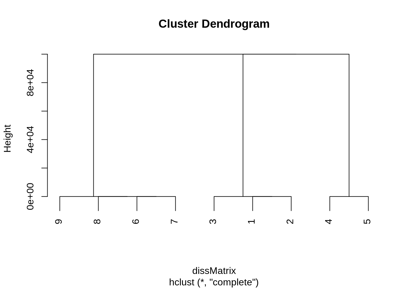
After merging 9-8-7-6, 3-1-2 and 4-5, there always exists a node that is not adjacent to another in one of the clusters. it follows that merging 9-8-7-6 and 3-1-2 or 9-8-7- and 4-5 is equivalent in terms of objective function and we will not necessarily retrieve the natural clustering. This is also mentionned in this other post. This is independent of the badnwith \(\sigma\) considered to create the dissimilarity matrix. Using simple linkage yields the same results as spectral clustering, but this might not always be the case with weighted edges.
Omitting the penalization of non-adjacent edges yields the same cluster assignment, albeit with a much smaller total cluster distance of 1.
Combinatorial optimization / unsupervised statistics - metrics
The following section departs from the graph-centric perspective used heavily above. It focuses on the difference between points based on a set of \(p\) features rather than the structure of the dissimilarity graph.
Intra-cluster distance
In order to group \(n\) points \(\{x_i\}\) where \(x_i \in \mathbb{R}^p\) into \(k=|C|\) homogeneous clusters, we may consider the total weighted intra-cluster distance. This is one of the most intuitive and commonly used metric. Consider the following distance functions:
\[d: \mathbb{R}^p \times \mathbb{R}^p \rightarrow \mathbb{R}_+\]
where
- \(d(x_i ,x_j)=d(x_j,x_i )\), \(d(x_i ,x_j)=0 \Leftrightarrow x_i = x_j,\)
- \(d(x_j,x_m) + d(x_m,x_i ) \leq d(x_j,x_i ), \forall x_j,x_i ,x_m.\)
If we assign weight \(\omega_i \in \mathbb{R}_+\) to the point \(i\), then \(\Omega_c = \sum_{i \in C_c} \omega_i\) is the total cluster weight and \(\mu_c= \frac{\sum_{i \in C_c} x_i \omega_i}{\Omega_c}\) is the total cluster average. Considering the popular squared Euclidean norm:
\[ \begin{align} d_2(x_i , \mu_c ) &= \left\lVert x_i - \mu_c \right\rVert_2^2 \\ &= \sum_{l=1}^p (x_{il} - \mu_{jl})^2 \end{align} \]
we then see that the total cluster intra-distance is simply the cluster weighted intra-variance:
\[ \begin{align} & \sum_{c = 1 }^{|C|} \frac{\Omega_c}{ \Omega } \sum_{i \in C_c } \left\lVert x_i - \mu_c \right\rVert_2^2 \omega_i \\ &= \frac{1}{ \Omega } \sum_{c = 1 }^{|C|} \Omega_c \sum_{i \in C_c } \left( \left\lVert x_i \right\rVert_2^2 + \left\lVert \mu_c \right\rVert_2^2 - 2 \left\langle x_i , \mu_c \right\rangle \right) \omega_i \\ &= \frac{1}{ \Omega } \sum_{c = 1 }^{|C|} \Omega_c \left( \sum_{i \in C_c } \left\lVert x_i \right\rVert_2^2 \omega_i + \Omega_c \frac{1}{\Omega_c^2} \sum_{i \in C_c } \sum_{j \in C_c } \left\langle x_i , x_j \right\rangle \omega_i \omega_j - 2 \frac{1}{\Omega_c} \sum_{i \in C_c } \sum_{j \in C_c } \left\langle x_i , x_j \right\rangle \omega_i \omega_j \right) \\ & = \frac{1}{ \Omega } \sum_{c = 1 }^{|C|} \sum_{i \in C_c } \sum_{j \in C_c } \left( \left\lVert x_i \right\rVert_2^2 \omega_i \omega_j - \left\langle x_i , x_j \right\rangle \right) \\ &=\frac{1}{ \Omega } \frac{1}{2} \sum_{c = 1 }^{|C|} \sum_{i \in C_c } \sum_{j \in C_c } \left\lVert x_i - x_j\right\rVert_2^2 \omega_i \omega_j \\ &=\frac{1}{ \Omega } \frac{1}{2} \sum_{c = 1 }^{|C|} \sum_{i \in C_c } \sum_{j \in C_c } d(x_i ,x_j) \omega_i \omega_j . \end{align} \]
The last expression is simply the (weighted) sum of the distances between all points within the clusters (scaled by \(\Omega^{-1}\), which is immaterial if we are optimizing). We divide by \(\frac{1}{2}\) because of the symmetry and to avoid double counting: \(d(x_i ,x_j) = d(x_j,x_i )\).
Given \(k\) clusters, consider the following equalities:
\[ \begin{align*} \underbrace{ \sum_{i =1}^n \sum_{j =1}^n d(x_i ,x_j)\omega_i \omega_j}_{total \, distance} & = \underbrace{ \sum_{c=1}^k \sum_{i \in C_c} \sum_{j =1}^n d(x_i ,x_j)\omega_i \omega_j}_{total \, distance} \\ & = \underbrace{ \sum_{c} \sum_{i \in C_c} \sum_{j \in C_c} d(x_i ,x_j)\omega_i \omega_j}_{within \, cluster \, distance} + \underbrace{ \sum_{c} \sum_{i \in C_c} \sum_{j \not\in C_c} d(x_i ,x_j)\omega_i \omega_j}_{between \, cluster \, distance} \end{align*} \]
It follows that minimizing the total within (intra) cluster distance is equivalent to maximizing the total between (inter) cluster distance since the total distance is a constant accross all partitions of points.
K-means algorithm
A popular algorithm for this type of problem is the k-means algorithm which iterates between assignment based on the nearest centroid and centroid update. At termination, a point belongs to cluster \(C\) if the distance from the centroid of that cluster is smaller than the distance to any other centroid. The final \(k\) centroids \(\{c_j\}_{j=1}^k\) induce the following clusters:
\[ C_i = \{x \in \mathbb{R}^p : d(x,c_i) \leq d(x,c_j) ,\forall j\neq i \}, \quad i =1,\cdots, k \]
It turns out that \(\{ C_k \}_{k=1}^K\) is precisely the Voronoi partitiongiven the poinst \(\{c_j\}_{j=1}^k\). For a finite set of points in Euclidian space, it will be convex since \(d(x,\mu_c) =\left\lVert x-\mu_c \right \rVert\) and \(\left\lVert x-\mu_c \right \rVert^2 = \left\lVert x \right \rVert^2 + \left\lVert \mu_c \right \rVert^2 - 2 \langle x,\mu_c\rangle\). Hence:
\[ d(x,\mu_c) \leq d(x,\mu_{c'}) \Leftrightarrow \frac{ \left\lVert \mu_c \right \rVert^2 - \left\lVert \mu_{c'} \right \rVert^2 }{2} \leq \langle x, \mu_c - \mu_{c'} \rangle \]
It follows that the Voronoi cell assocaited with centroid \(c\) can be represented as the following finite intersection of halfspaces, which is precisely a (convex) polyhedron:
\[ \bigcap_{c' \neq c} \left\lbrace x: \frac{ \left\lVert \mu_c \right \rVert^2 - \left\lVert \mu_{c'} \right \rVert^2 }{2} \leq \langle x, \mu_c - \mu_{c'} \rangle \right \rbrace \]
Cluster diameter
For any cluster \(C_c\), we define the cluster diamenter as the maximum distance between any points in the cluster4:
\[ D(C_c) = \max_{i,j \in C_c} d(x_i ,x_j) \]
This metric is also known as the maximum intra-cluster distance and is implicitely considered when using standard agglomerative hierarchical clustering with complete linkage.
We can then minimize the following value over all clusters:
\[ D(G) = \max_{c = 1\cdots k } D(C_c) \]
Using this metric will ensure no large clusters exists, but could also produce unbalanced clusters of varying size. It is also possible that on average, clusters be larger than the average cluster size if total intra-cluster distance is used.
This is the metric considered in professors Contardo and Aloise paper. It plays a fundamental role in their column generation procedure and helps them solve very large instances with a few thousand variables.
A markov Chain is essentially a simple discrete stochastic process \(\{X_k\}\) over a given state space \(S=\{1,\cdots,n\}\) with the fundamental property that \(P(X_{t+1}=j | X_{t}=i_0,X_{t-1}=i_{1}, \cdots , X_{t-K}=i_{K} \} = P(X_{t+1}=j | X_{t}=i_0)\) for \(j,i_k \in S\). An irreducible markov Chain is set of nodes/states that may be reached in a finite number of steps from any node in that set. A finite Markov chain contains a finite number of states/nodes. For an aperiodic Markov chain, there exists \(N \in \mathbb{N}\) such that \(P_{ii}^n > 0\) for all \(n\geq N\) and all \(i\). In other words, it is possible to return to any state in any number of steps \(n \geq N\). There exists a wealth of references on the subject. Consider for instance these notes.↩
Although it would be preferable to add Inf for these particular pairs, stats::hclust does not handle NAs NULLs of Infs well. We therefore have to settle for soft constraints and large finite values that could represent an upper bound on the total weighted intra cluster distance for example.↩

Social/Complex Networks - metrics
A central theme in social network theory is the study of the relationships between individuals and the structure of the resulting relationship graph. The following representative metrics consider the density of edges within groups of points relative to the density of edges between different groups in order to determine the existence of communities (clusters).
Although this litterature is primarily concerned with the structure of the graph rather than distance between points based on different features, it shares many caracteristics with other more traditional clustering methods
Modularity
Modularity is a measure of the propensity of groups of nodes to be densely connected within the given cluster, but sparsely connected with other groups of nodes. It is based on the discrepancy between the number of edges between different clusters and the expected number of edges based on a random graph model. This random graph model supposes that we keep the same number of edges and nodes, but that we randomly reconfigure the edges based on the the degrees \(d_i\) of each node \(i \in V\).
For any \(i\in V\), the probability that an edge with endpoint \(i\) is rewired to \(j \in V\) depends only on the degree of \(j\):
\[P_{i , j} = \frac{d_j}{\sum_{j\in V} d_j}\] If \(E(i,j)\) represents the number of edges between \(i\) and \(j\), the expected number of edges between \(i\) and \(j\) is therefore (allowing self loops):
\[ \begin{array}{ll} \mathbb{E}[E(i,j)] &= \displaystyle \sum_{s=1}^{d_i} P_{i , j} \\ & = \displaystyle\sum_{s=1}^{d_i} \frac{d_j}{\sum_{j\in V} d_j} \\ & = \displaystyle \frac{d_i d_j}{\sum_{j\in V} d_j} \\ &= \displaystyle \frac{d_i d_j}{2 m} \end{array} \]
where the last line follows from the fact that \(\sum_{i \in V} d_i = 2m\).
The modularity of an edge \((i,j)\) is then defined as the difference between the actual number of edges and the expected number of edges from the random reconfiguration if the 2 edges lie in different clusters:
\[ Q_{ij} = \left( A_{ij} - \displaystyle \frac{d_i d_j}{2 m} \right) I_{i \in C_{a}, j \in C_{b}, a\neq b } \]
We then define the modularity of a graph as the sum over all pairs of nodes that lie in different clusters, divided by \(2m\) to ensure that the graph modularity lies within \([-1,1]\):
\[ \begin{array}{ll} Q &= \displaystyle \frac{1}{2m} \sum_{i \in V} \sum_{j \in V} Q_{ij} \\ \end{array} \]
For the toy example, we see that modularity is relatively low when considering the natural bipartition given by the simple connected components. In this case, there exists too few edges within the clusters. Partitioning the graph into the three cliques \(K_2, K_3\) and \(K_4\) considerably increases the metric.
Clustering coefficient
The clustering coefficient is another popular measure of the density of the graph. It measures the propensity of 2 neighbourhing nodes to share another common neighbour. In other words, it is a measure of the number of triangles in the graph. This is closely related to the concetp of triadic closure in sociology.
This metric is instrumental in defining properties of the Watts-Strogatz model for small-world networks. Small world networks are random graphs with high clustering coefficients and low average shortest paths. They were introduced with the goal of representing various real social structures that could not be explained by traditional random graph theory.
The (local) clustering coefficient for node \(i\) is defined as:
\[ \rho_i = \frac{ |\{ e_{jk} \in E : v_j, v_k \in N_i \}| } { \tau_i }, \]
where the numerator \(|\{ e_{jk} \in E : v_j, v_k \in N_i \}|\) is equal to 3 times the number of triangles in \(G\). A triangle is an induced subgraphs on 3 vertices with 3 edges, i.e. \(K_3\). Each triangle is counted 3 times, once for each of its vertices.
The denominator \(\tau_i\) is an upper bound for 3 times the number of triangles on the neighbours of \(i\):
\[ \tau_i = \begin{cases} \frac{d_i (d_i-1) }{2} = {n \choose 2} & \text{ if } G \text{ is undirected } \\ d_i (d_i-1) = {n \choose 2}2=\frac{n!}{(n-2)!} & \text{ otherwise. } \end{cases} \]
For the graph above, we see that the clustering coefficient is relatively high. However, we note that although interesting, this metric is invariant to different partitions.
As we can see from the output, the coefficient is maximized when the set of neighbourhds forms a clique. We also observe that it is only defined for nodes with at least 2 neighbours.
Measures based on random walks
There exists other works that consider metrics based on the structure of the relationship graph. For instance, the work of Pons and Latapy considers a metric exploiting properties of random walks. The intuition is that short random walks on a graph have a high tendency of staying within the same cluster of densely connected nodes.
The authors consider unweighted graphs and define the random walk structure by assuming that given a current node \(i\), the probability of transiting to any other node \(j\) is \(p_{ij}=\frac{A_{ij}}{d_i}\), which is 0 if \(j\) is not a neighbour of \(i\) and \(d_i^{-1}\) otherwise. We conclude that the random walk has exactly the same probability of transiting to any neighbour and \(\sum_j p_{ij} = d_i\) so this indeeed defines a probability. The transition matrix can then be compactly defined as:
\[ P= D^{-1}A \]
Computing the transition matrices in \(t \in \mathbb{N}\) steps can be done through matrix multiplication: \(P^t = (D^{-1}A)^t\). It follows that \(P_{i}^t\) is the \(i^{th}\) row of \(P^t\) and defines the probability of transiting to any other node in \(t\) steps after starting from node \(i\).
Here is an example with \(t \in \{ 1,10,1001 \}\) for the graph presented above:
We notice that \(\lim_{t \rightarrow \infty} p_{ij}^t\) is converging to a constant matrix with a particular structure.
Indeed, the graph consists of 2 finite irreductible Markov chains 1 which correspond to each of the 2 connected components. The chain composed of 1-2-3 and 6-7-8-9 is aperiodic which implies the existence of a stationay distribution \(\pi\) such that \(\pi P = \pi\). Indeed we can verify that for all \(j \in \{1,2,3,6,7,8,9\}\):
\[ \begin{align*} \lim_{t \rightarrow \infty} p_{ij}^t& = \frac{d_j}{\sum_k d_k} , \forall i\\ & = \pi_j \end{align*} \]
indeed represents the desired stationary distribution. In this case, the probability of eventually ending up at node \(j\) only depends on the degree of \(j\), regardless of the starting node \(i\). Notice that this stationary probability distribution is precisely the probability used to define modularity above.
For the other chain composed of 4 and 5, the period is 2, meaning that we can only return to a given node after visiting 2 edges and it is impossible to find such stationary distribution. Ineed, we notice that after \(t\) even steps, the
while for \(t\) odd, we have the different permuted matrix:
Therefore, the probability of ending up at node \(j\) always depends on the starting node \(i\), which was not the case of the other aperiodic chain. If \(i=j\), then we can only return to \(j\) in an even number of steps, otherwise an even number of steps is required.
Although interesting, this analysis is only meant to increase our understanding of the probability model underlying the clustering algorithm. The existence of a stationary distribution is not required. The authors rather exploit the fact that for sets of connected nodes it makes sense to group nodes into clusters based on the discrete probability distribution \(P_i^t\).
As can be gleaned from the analysis above, for high \(t\), \(P_i^t\) only depends on the degree of nodes and so does not provide meaningful information for clustering purposes. For low \(t\) however, the output above suggests that it has a tendency to recover the natural 1-2-3, 6-7-8-9 and 5-7 clusters as the row vectors of \(P^t\) are similar within these groups. More specifically the authors use the following distance to compare transition probabilities: :
\[ d_{ij}^t=\lvert \lvert D^{-1/2} (P_i^t-P_j^t) \lvert \lvert_2 \]
They then propose a greedy agglomerative algorithm which is essentially one of the variants of the classical hierarchical clustering algorithm to construct the dendrogram.