
Introduction
The big day’s approaching fast and you need to find a way to find a good seating plan that will please all your hosts? Fear not, I have the solution for you. If you manage to pull through all the mathematical models and code, you’ll have a way to seat your friends together while avoiding any disputes between enemies and adequately mixing high and low energy hosts.
Here’s the plan. You’ll need to:
- Assign \(n\) guests to \(K\) tables
- Tables have capacities
- Guests have preferences
- Some guests cannot be seated with others
- Some guests must be with others
- Some guests can have more weight than others
The goal is to:
- Satisfy all constraints
- Maximize some metric (total intra-cluster affinity in this case)
Lucky you, this problem can be cast as a constrained clustering algorithm
Guest graph
First, let’s take a look at a graph representing all the hosts as well as their relationships:
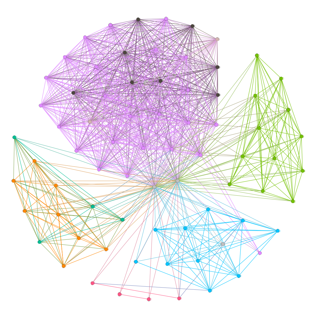
Guest Graph
Each node represents a guest, the edges indicate that the guests know each other and the colors represent specific groups of friends or families.
It was produced using the excellent and open-source gephi software for graph visualization and inspection. The actual embedding/drawing was created using the Fruchterman-Reingold algorithm, but there exists other that will provide different figures that can highlight different structures. Even without any coloring, initial clusters of guests immediately appear and we can get an idea of the centrality of certain nodes.
Creating the input for Gephi
Here’s some sample R code explaining how this graph could be created. The binary coding can then be used to color the nodes and assign a guest to a specific group. The cluster code is unique and a guest can belong to multiple groupes. For instance, a gues belonging to Family1 and Family2 will have a unique code of 4+8=12.1
writeGuestGraph <- function( ){

  #adjmatrix is an nXn matrix/df with a 1 in position ij if guest i knows guest j and 0 otherwise
  adjmatrix <-   readAdjmatrix( )

  #dfFeaturesGuests is an nXp matrix/df where each of the n guests has p features including a 0/1 coding for family membership (could also add age, sex, hobbies, etc)
  dfFeaturesGuests <- readFeatureMatrix()

  #Use igraph to create the initial graph with the adjacency matrix
  guestGraph <- igraph::graph_from_adjacency_matrix(adjmatrix )

  #as_long_data_frame outputs the edge list
  dfEdges <- igraph::as_long_data_frame( guestGraph )
  dfNodes <- data.frame( Label = rownames( adjmatrix ) ,
                         Id = 1:nrow(adjmatrix))

  #Add features to the guests/nodes (namely use for coloring)
  dfNodes <- left_join( dfNodes,
                        dfFeaturesGuests,
                        by='Label')

  #Assign a unique number to each possible cluster by codifying in binary
  #(Ok since the features used for clustering are all 0-1)
  dfNodes %<>% dplyr::mutate(  Cluster = Friends1*2^0+
                                 Friends2*2^1+
                                 Family1*2^2+
                                 Family2*2^3+
                                 Family3*2^4+
                                 Family4*2^5 )


  #The gexf format only takes 2 columns

  #Watch out! use the correponding node indexing in both nodes and edge df (does it start at 0 or not?)
  #Also watch out for the order of Id and Label => the 1st column is always taken to be the ID
  gexfGraph <- write.gexf(nodes= dfNodes %>% dplyr::select(Id, Label)  ,
                          edges= dfEdges %>% dplyr::select(from, to )  ,
                          nodesAtt = dfNodes %>% dplyr::select(  -Label, - Id )
  )


  #Output the resulting graph
  #Don't forget the extension otherwise gephi will complain
  print(gexfGraph, file = "Output/guestGraph.gexf")

}
It could be possible to use a slighlty more refined version where the edge weights represent affinity between guests and are reals in \([0,1]\) rather than simply binary. The edge weights can then be adjusted accordingly in the embedding.
Mathematical program
Using the preceding graph above, we could simply group cliques of guests at the same table (groups of guests that each know everyone else in that group). This naive approach could work, but ignores the fact that tables have a fixed capacity. It might also be useful to ensure that certain guests that know each other are not at the same table or to mix family and friends.
In order to devise such an assignment, we formalize the problem as a clustering problem where we seek to maximize the total affinity within each cluster (table/group of guests):
##Original mathematical program
We seek an optimal solution to the following (non-linear integer) mathematical program (you might want to flip your mobile device): 2
\[ \begin{align*} & ( {\text{Total weighted affinity}}) & \max_{x} & \sum_{c \in C } \sum_{i \in I} \sum_{j \in I; j \neq i} a_{ij} x_{ic} x_{jc} {\omega}_i {\omega}_j \label{eq:objValue} \\ % % & ( {\text{Each guest assigned to exactly one table}} ) & \text{s.t.} & \sum_{c \in C} x_{ic} = 1 &&\forall i \in I \label{eq:oneCluster} \\ % % % % & ( {\text{Table capacity}} ) & & \sum_{i \in I} x_{ic} \leq \tau_c &&\forall c \in C \label{eq:clusterCapacity} \\ % % % % & ( {\text{Must-link constraints}}) & & x_{ic} = x_{i'c} && \forall c \in C , (i,i') \in P_O \label{eq:mustLink} \\ % % & ( {\text{Cannot-link constraints}}) & & x_{ic} + x_{i'c} \leq 1 && \forall c \in C , (i,i') \in P_N \label{eq:cannotLink} \\ % % % % & ({\text{Binary assignment of cluster}} ) & & x_{ic} \in \{0,1\} && \forall i \in I; c \in C \label{eq:nonNegativeIntegersX} \end{align*} \]
where:
- \(I=\{1,\cdots, n\}\) : set of \(n\) guests
- \(C=\{1,\cdots,K\}\) : set of \(K\) tables
- \(\tau_c\) : capacity of table \(c\)
- \(a_{ij}\) : affinity between guests \(i\) and \(j\)
- \(P_O, P_N \subset I \times I\): pairs of guests that must and cannot be together
- \(\omega_i\) : weight of guest \(i\)
and:
- \(x_{ic}\) : binary variable indicating if guest \(i\) is assigned to table \(c\)
Solving this mixed integer non-linear formulation seems like a daunting task. As mentionned in my other post on clustering, clustering without constraints is alreay NP-hard. Adding constraints only increases this intractability. It therefore seems unlikely that we can find a tractable formulation at all. However, we can still try to improve this formulation to make more amenable to existing mathematical programming solvers.
Bilinear terms
If we seek to maximize the sum of intra cluster affinity, then the objective is a linear combination of bilinear terms:
\[\sum_{c \in C} \sum_{i \in I} \sum_{j \in J; j\neq i} a_{ij} \underbrace{x_{ic} x_{jc}}_{\text{bilinear}} \omega_i \omega_j\]
We want to “linearize” the bilinear (nonlinear) term. If we know that both variables are bounded, i.e. \(\exists a<b\) s.t.
\[x,y \in [a,b]\]
then we can find valid (linear) inequalities that bound the function and provide a bound on the value of the true problem. Indeed, any solution of the initial problem is also feasible for the new relaxed problem with same objective value. The latter problem is therefore overoptimistic and provides an upper bound since this is a maximization problem:
\[ \begin{align} 0 &\leq (a-x)(y-b) = ay -ab - xy + xb \\ & \Leftrightarrow xy \leq ay -ab + xb\\ & \Leftrightarrow xy \leq y \text{ since } a=0, b=1 \end{align} \]
Repeating the same analysis for the remaining 3 possibilities \((x-b)(y-b) \geq 0 , (a-x)(a-y) \geq 0 , (x-b)(y-b) \geq 0\), we get 4 linear inequalities.
These sets of inequalities are known as McCormick inequalities.
Bilinear terms - pictures
If equations don’t appeal to you, then perhaps this 3D visualization (created using the excellent plot.ly3 R library) will (touch the figure if nothing appears):
Here’s the R code that was used to produce this figure by the way:
library(plotly)
library(htmlwidgets)

library(tidyr)
library(magrittr)
library(dplyr)


x <- seq(0,1,0.01)
y <- seq(0,1,0.01)
z <- matrix( nrow= length(x), ncol=length(y))
hyperplane1 <- matrix( nrow= length(x), ncol=length(y))
hyperplane2 <- matrix( nrow= length(x), ncol=length(y))
hyperplane3 <- matrix( nrow= length(x), ncol=length(y))

for(i in 1:length(x)){
  for (j in 1:length(y)){
    z[i,j] <- x[[i]]*y[[j]]
    #First linear constraints z>=x+y-1
    hyperplane1[i,j] <- max(0, x[[i]] + y[[j]] -1 ) #truncate at 0 since negative segments do not interest us
    #z<= x
    hyperplane2[i,j] <- x[[i]]
    #z<= y
    hyperplane3[i,j] <- y[[j]]
  }
}


plotlyPlot <- plot_ly(x=~x,y=~y) %>%
  add_surface(z=~z, opacity =0.8,colorscale  =  list(c(0,"rgb(255,112,183)"),c(1,"rgb(128,0,64)") ) ) %>%
  add_surface(z=~hyperplane1, opacity =0.5) %>%
  add_surface(z=~hyperplane2, opacity =0.5) %>%
  add_surface(z=~hyperplane3, opacity =0.5) %>%
  layout(title = 'Bilinear function and 3 bounding hyperplanes')

plotlyPlot

htmlwidgets::saveWidget(widget=plotlyPlot, "bilinear.html" , selfcontained = FALSE)
Linearized Mathematical Program
We can then use these McCormick inequalities to linearize the non-linear bilinear terms \(x_{ic} x_{jc}\) in the objective of our initial mathematical program:
\[ \begin{align} & ( {\text{Total weighted affinity}}) & \max_{x,w} & \sum_{c \in C } \sum_{i \in I} \sum_{j \in I; j\neq i} a_{ij} w_{ijc} {\omega}_i {\omega}_j \label{eq:objValue2} \\ % % & ( {\text{Each guest assigned to 1 table}} ) & \text{s.t.} & \sum_{c \in C} x_{ic} = 1 &&b\forall i \in I \label{eq:oneCluste2r} \\ % % % % & ( {\text{Table capacity}} ) & & \sum_{i \in I} x_{ic} \leq \tau_c &&b\forall c \in C \label{eq:clusterCapacity2} \\ % % % % & ( {\text{Must-link constraints}}) & & x_{ic} = x_{jc} && \forall c \in C ; (i,j) \in P_O \label{eq:mustLink2} \\ % % & ( {\text{Cannot-link constraints}}) & & x_{ic} + x_{jc} \leq 1 && \forall c \in C ; (i,j) \in P_N \label{eq:cannotLink2} \\ % % % % & ( {\text{McCormick 1}}) & & w_{ijc} \leq x_{ic} && \forall i,j \in I; c \in C \label{eq:mcCormick1} \\ % % % % & ( {\text{McCormick 2}}) & & w_{ijc} \leq x_{jc} && \forall i,j \in I; c \in C \label{eq:mcCormick2} \\ % % % % & ( {\text{McCormick 3}}) & & w_{ijc} \geq x_{ic}+ x_{jc} - 1 && \forall i,j \in I; c \in C \label{eq:mcCormick3} \\ % % % % & ( {\text{Binary assignment of cluster}} ) & & x_{ic} \in \{0,1\} && \forall i \in I; c \in C \label{eq:nonNegativeIntegersX2} \\ % % % % & ( {\text{Non-negative linearizing variables}} ) & & w_{ijc} \geq 0 && \forall i,j \in I; c \in C \label{eq:nonNegativeIntegersW} \end{align} \]
We have eliminated the bilinearities, but we are still left with a rather hard integer problem. Moreover, the linearization has introduced \(n^2K\) new variables and \(O(n^2K)\) constraints. We can try to alleviate this issue by using the must-link constraints to group guests together into fixed clusters.
Linearized Mathematical Program with grouped guests
We can substitute the must-link constraints directly in the objective and replace \(I\) by \(\mathcal{I} = \mathcal{I}' \cup \mathcal{I}''\) where
\[\mathcal{I}' = \{ \{i \}: i \in I ; (i,j) \not \in P_0, \forall j \in I \}\] represents the guests that are not part of any must-link constraints and
\[\mathcal{I}'' = \bigcup_{F \in \mathcal{F}} \{ \{i_{1}, \cdots, i_{|F|} \}: i_{l} \in I \cap F \}\]
represents “meta guests” or clusters of guests that must be seated together. \(\mathcal{F}\) are the connected components in the graph with edges \(P_0\) and nodes having at least one endpoint in \(P_0\). Note that \(\mathcal{I}'\) and \(\mathcal{I}'\) are now treated as collections of sets and \(\mathcal{I}', \mathcal{I}'' \subset P(I)\).
If we denote \(\bar{n} = |\mathcal{I}|\), then the problem has less decision variables than the previous since \(\bar{n} < n\) if \(|P_O |> 1\). In other words if we must merge at least 2 guests, then we have at least one less “meta guest” or cluster of guests to assign to tables.
Once we have grouped guests into a new meta-guest we must adjust the affinity between that cluster and the other cluster guests. In our simple case, this is simply the average affinity:
\[ \begin{align} \bar{a}_{KL} = \frac{\sum_{i \in K }\sum_{j \in L} a_{ij} \omega_i \omega_j }{\bar{\omega}_K \bar{\omega}_L } & K \in \mathcal{I}, L \in \mathcal{I} \\ \end{align} \]
where for meta guest \(K \in \mathcal{I}\), \(\bar{\omega}_K = \sum_{i \in K} \omega_i\) represents the total weights of the guests in that group. The table capacities must be modified by considering: \(n_K = |K|\), the number of guests in cluster \(K\), where \(\sum_{K \in \mathcal{I}} n_K = n\).
The cannot link constraints are replaced by a new set of constraints \(P_N'\) where 2 clusters cannot be grouped together as soon as there exists one guest in each that cannot be seated together.
\[ \begin{align*} & ({\text{Total weighted affinity}}) & \max_{x,w} & \sum_{c \in C} \sum_{I \in \mathcal{I}'} \sum_{J \in \mathcal{I}'; J\neq I} \bar{a}_{IJ} w_{IJc} {\bar{\omega}}_I {\bar{\omega}}_J \label{eq:objValue3} \\ % % & ({\text{Each guest assigned to exactly one table}} ) & \text{s.t.} & \sum_{c \in C} x_{Ic} = 1 &&\forall I \in \mathcal{I}' \label{eq:oneCluste22} \\ % % % % & ({\text{Table capacity}} ) & & \sum_{I \in \mathcal{I}'} n_I x_{Ic} \leq \tau_c &&\forall c \in C \label{eq:clusterCapacity3} \\ % % % % & ({\text{Cannot-link constraints}}) & & x_{Ic} + x_{Jc} \leq 1 && \forall c \in C ; (I,J) \in P_N' \label{eq:cannotLink3} \\ % % % % & ({\text{McCormick 1}}) & & w_{IJc} \leq x_{Ic} && \forall I,J \in \mathcal{I}; c \in C \label{eq:mcCormick12} \\ % % % % & ({\text{McCormick 2}}) & & w_{IJc} \leq x_{Jc} && \forall I,J \in \mathcal{I}; c \in C \label{eq:mcCormick22} \\ % % % % & ({\text{McCormick 3}}) & & w_{IJc} \geq x_{Ic}+ x_{Jc} - 1 && \forall I,J \in \mathcal{I}; c \in C \label{eq:mcCormick32} \\ % % % % & ({\text{Binary assignment of cluster}} ) & & x_{Ic} \in \{0,1\} && \forall I \in \mathcal{I}; c \in C \label{eq:nonNegativeIntegersX22} \\ % % % % & ({\text{Non-negative linearizing variables}} ) & & w_{IJc} \geq 0 && \forall I,J \in \mathcal{I}; c \in C \label{eq:nonNegativeIntegersW2} \end{align*} \]
if we wish to compute the true optimal value, we may add the constant \(\sum_{(i,j) \in P_O^k} a_{ij} \omega_i \omega_j\) (the total affinity of guests that must be placed together), but this is immaterial to finding the optimal solution since this is constant regardless of the assignment.
Implementation
Now that’ve properly defined the problem, let’s take a look at the set of tools available to solve the problem and avoid infuriating your future wife with mathematical formalism.
Data
It would be possible to send out a form to all guests and ask them a few question such as their age, sex, interests, membership to a particular group and hobbies in other to form a \(n\times p\) feature matrix. This feature matrix could then be used to create a simple \(n\times n\) affinity/dissimilarity/distance between guests. This could namely be interesting to implement for the folks at greenvelope4.
For our present problem instance however, I simply manually filled in the lower diagonal of a \(n\times n\) affinity matrix (assuming affinity is symmetric) manually using discrete values in \(\{1,2,3,4\}\) and coding cannot-link constraints as \(-1\) and must-link constraints as \(5\). Here’s a sample of the dataset:
| X | Guest1 | Guest2 | Guest3 | Guest4 | Guest5 | Guest6 | Guest7 | Guest8 | Guest9 |
|---|---|---|---|---|---|---|---|---|---|
| Guest1 | NA | NA | NA | NA | NA | NA | NA | NA | NA |
| Guest2 | 5 | NA | NA | NA | NA | NA | NA | NA | NA |
| Guest3 | 3 | 3 | NA | NA | NA | NA | NA | NA | NA |
| Guest4 | 3 | 3 | 5 | NA | NA | NA | NA | NA | NA |
| Guest5 | 2 | 2 | 2 | 2 | NA | NA | NA | NA | NA |
| Guest6 | 2 | 2 | 2 | 2 | 5 | NA | NA | NA | NA |
| Guest7 | 1 | 1 | 1 | 1 | 1 | 1 | NA | NA | NA |
| Guest8 | 1 | 1 | 1 | 1 | 1 | 1 | 5 | NA | NA |
| Guest9 | 1 | 1 | 1 | 1 | 1 | 1 | 4 | 3 | NA |
| Guest10 | 1 | 1 | 1 | 1 | 1 | 1 | 3 | 3 | 5 |
Model in R with ompr
I also had a try at the ompr package in R. This package provides an intuitive way to model mixed-integer linear mathematical programs algebraically. It then interfaces with a given solver that solves the problem.
  library(ompr) #ompr does the algebraic model + then converts to matrices and format a solver can understand (e.g. mps)
  library(ompr.roi)
  library(ROI.plugin.glpk) #glpk is the open source solver for linear and integer optimization => this is a sh** solver


  model <- MIPModel() %>%

    # 1 iff i gets assigned to warehouse j
    add_variable(x[i, j], i = 1:nGuests, j = 1:numTables, type = "binary") %>%
    #Additional variable for McCormick relaxation
    #Only use half the vars since w_i,ip,j = 1 iif i and ip are assigned to j (order or i and ip is irrelevant, only set membership important)
    add_variable(w[i, ip, j],
                 i = 1:nGuests,
                 ip = 1:nGuests,
                 j = 1:numTables,
                 i < ip ,  #symmetry
                 type = "continuous", lb = 0, ub = 1) %>%

    #All w_i,ip,j vars and associated constraints are only defined for i<ip due to symmetry
    #This reduces the number of w vars by 2 + number of constraints involving w's by 2
    #e.g. x_1j + x_3j <= 1 and x_3j + x_1j  <= 1 are equivalent

    #Constraints for McCormick: 1
    add_constraint( w[i, ip, j] >= 0 , i = 1:nGuests, ip=1:nGuests, j = 1:numTables, i<ip ) %>%
    #Constraints for McCormick: 2
    add_constraint( w[i, ip, j] >= x[i, j] + x[ip, j] - 1 , i = 1:nGuests, ip=1:nGuests, j = 1:numTables, i<ip ) %>%
    #Constraints for McCormick: 3
    add_constraint( w[i, ip, j] <= x[i, j] , i = 1:nGuests, ip=1:nGuests, j = 1:numTables, i<ip )  %>%
    #Constraints for McCormick: 4
    add_constraint( w[i, ip, j] <= x[ip, j], i = 1:nGuests, ip=1:nGuests, j = 1:numTables , i<ip ) %>%


    #Constraint - each guest assigned to exactly one cluster
    add_constraint( sum_expr(x[i, j] , j = 1:numTables ) == 1 , i = 1:nGuests ) %>%

    #Constraint - respect the table capacities
    add_constraint( sum_expr(x[i, j] , i = 1:nGuests ) <=  tableCapacity ,  j = 1:numTables)

  # ... other code to validate constraints ...

  ## Set the objective ##

  #We should MAXIMIZE the affinity, bu MINIMIZE the featureDistance
  sensObj <- ifelse( all( affinityMatrix[!is.na(affinityMatrix)] == featureDistance[!is.na(featureDistance)] ) ,
                     "max", "min" )

  print(paste0("This is the obj we are optimizaing: ", sensObj))

  #Objective : This is the linear relaxation of the true problem
  #Total intra-cluster variance (divide by 1/2 to avoid double counting)
  model %<>% set_objective( sum_expr(featureDistance[i, ip] * w[i, ip, j],
                          i = 1:nGuests,
                          ip= 1:nGuests,
                          j = 1:numTables ,
                          i< ip )
                 , sense = sensObj)


  print("Model summary before solving: ")
  print(model)

  #Solve the model#
  system.time(
    result <- solve_model(model, with_ROI(solver = "glpk" ,verbose=T))
  )

  #Inspect the solution
  if( result$status == "optimal" ) { dfSolution <- inspectSolution( result, affinityMatrix)
  }else {print("Error, model not solved to optimality"); return(NULL)}
As can be gleaned from the preceding R snippet, ompr provides a rather flexible and convenient way to model a mathematical program in R. However, I was limited by the use of the open source glpk solver. I therefore tried another approach.
Model in AMPL
The easiest and fastest way for me to get access to more performant solvers was to used the all-powerful CPLEX solver through the Neos infrastructure. in order to do so, I replaced ompr with AMPL. AMPL is a more flexible mature and flexible algebraic modeling language than ompr. It provides support for non-linear problems as well as a host of different solvers. it requires 3 files: a model file, a data file and a run file:
The syntax is reminiscent of ompr ad is very close to the initial mathematical formalism presented above.
Solving the model
Neos server
I used the Neos server to run the AMPL model. This is a server that hosts many solvers for different type of optimization problems. You submit the mode, data and execution (run) file with your adress, it will solve the model for you and send you a message with the solution.
Here are a couple of snapshots of the different steps required (some of the data has been anonymised):
Results
Unsurprisingly, the final solution is very far from the optimum. This is to be expected with such a sloppy and loose formulation. Even with such a simple instance, the solver fails to find the solution within the alloted time.
Thankfully (!), CPLEX provides the best feasible integer solution before reaching the timeout of if it receives a keyboard interrupt. This was the final solution is used.
For the sake of completeness and to show that this was not a complete waste of your time, here’s a sample of the actual solution:
| guestName | cluster |
|---|---|
| Guest48_Guest49 | 1 |
| Guest1_Guest2 | 1 |
| Guest69_Guest70 | 1 |
| Guest33 | 1 |
| Guest38_Guest39 | 1 |
| Guest11 | 2 |
I your wife still wants to marry you after enduring all this rambling about linearizations and clustering then you know you’ve found the one. It’s also a mystery how you can still manage to have friends and family to actually seat at these tables.
Further work
Jokes aside, a better approach would be to use column generation or at least better heuristic like VNS. If you’re serious about this stuff, then I highly recommend checking out professor Contardo publications and Aloise’s publications.
Note on anonymising the data
Check out the following elegant solution on SO to replace a list of names by another. In this case, I simply create 2 text files, the first “listA” is a copy-past of the list of original names from my .csv while the second “listB” is a list of Guest1, Guest2, etc. Each of these entries are seperated by newlines, but are unquoted (this is really just a copy-paste from open office spreadsheet.)5
paste -d : listA listB | sed 's/\([^:]*\):\([^:]*\)/s%\1%\2%/' > sed.script
sed -f sed.script affinites.csv > newAffinites.csv
It’s possible to visualize the graph (embedding) using igraph’s built-in visualization tools, but Gephi offers several↩
If you want a static version, check out this pdf version of the Mathematical programming formulation↩
If you don’t know them already, I highly recommend that you check them out. Plot.ly provides excellent interfaces in R, Python, Matlab, etc. Best of all, the compagny comes from Montréal!↩
For those interested, greenveloppe provides paid services to send and track invitations to guests for special occasions like weddings.↩
Watch out for special characters (e.g. è) and delimites (e.g. “-”)↩
