Definitions and assumptions

Spatial interpolation is performed on either extensive or intensive geographical variables. Extensive variables can be meaningfully aggregated over regions by summing over them. Important examples of such variables include population, number of English speakers and other count variables. ¹

On the other hand, intensive variables, which may be unitless, cannot be aggregated through summation. Examples include prevalence of low income on a scale of 1 to 100, proportion of women over 65 and after tax income per capita.

This post only considers extensive variables, but the methodologically can easily be extended to intensive variable as well. For simplicity, it also assumes that for each layer, the polygons partition the entire area of study into disjoint sets (usually true in practice) and that the union of both sets is the same (usually not the case in practice).

Fundamentals

Interpolating one variable from a given polygon layer to another can be done by refining both geometries and taking their intersections as shown in the figure below.

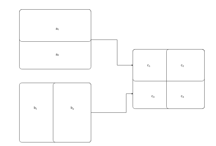
Refining the geometries through intersection

Once this intersection is computed, we can determine the following undirected graph of polygon correspondance:

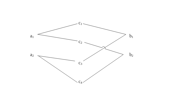
Tripartite graph illustrating the relationship between polygons from both layers

We abuse notation and use the same notation to refer to both the original polygons and the nodes in the graph. We denote \(A,B\) and \(C\) the set of nodes associated with polygons in the source, target and intersected layers respectively. We also use the lower case \(a,b,c\) to differentiate between the three layers.²

Having defined this correspondance, we can set up the interpolation by identifying a non-negative weighting variable \(\kappa\). This \(\kappa\) weight often corresponds to the area of the polygons in the refined intersected geometry, but we will explore other choices. We then define the weight of polygon \(i\) in the refined geometry as:

\[ w_{i}^c= \frac{\kappa_i^c}{\sum_{j \in N(p_a(i))} \kappa_j^c} \]

where \(p_a(i) \in A\) and \(p_b(i) \in B\) represent the unique associated parent/neighbour of node \(i \in C\) in each layer and \(N(k) \in A \cup B \cup C\) is the neighbourhood of node \(k\) in the tripartite graph.

Once this convex combination has been defined, we can interpolate any extensive variable \(v\) that is constant over polygons from layer \(a\) to \(c\) by taking:

\[ v_i^c = v_{p_a(i)}^a w_{i}^c \]

Finally, we can interpolate back to any polygon \(j \in B\) in the target layer by taking:

\[ v_j^b = \sum_{i \in N(j)} v_i^c \]

If \(\sum_{i \in N(k)} w_i^c =1, \forall k\) and every geometry in the intersection is associated to exactly 1 polygon in the source and target layers, then :

\[ \begin{align} \sum_{j \in B} v_j^b &= \sum_{j \in B} \sum_{i \in N(j)} v_i^c \\ &= \sum_{k \in A} \sum_{i \in N(k)} v_{p_a(i)}^a \frac{\kappa_i^c}{\sum_{j \in N(p_a(i))} \kappa_j^c} \\ &= \sum_{k \in A} v_{k}^a \sum_{i \in N(k)} \frac{\kappa_i^c}{ \sum_{j \in N(k)} \kappa_j^c} \\ &= \sum_{k \in A} v_{k}^a \end{align} \]

which means that the sum of \(v\) is preserved.

In reality, the problem is more complicated since the geometries rarely match perfectly. Even if the geographical atoms considered by authoritative sources like Statistics Canada stay the same, it is still possible that small tweaks to polygon boundaries occur, for instance to improve alignment with roads or water bodies. These incongruent geometries imply that without any adjustment, the sum of the interpolated variable is different in the two layers.

Area

The first and simplest approach consists in using the area of the polygons by computing st_area(geom). This makes sense if the variable we are trying to interpolate is uniformly distributed over the polygon. For population, this does not necessarily make sense. Indeed the dissemination area polygons used by Statistics Canada are designed to have a relatively similar population so that large polygons correspond to sparsely populated areas.

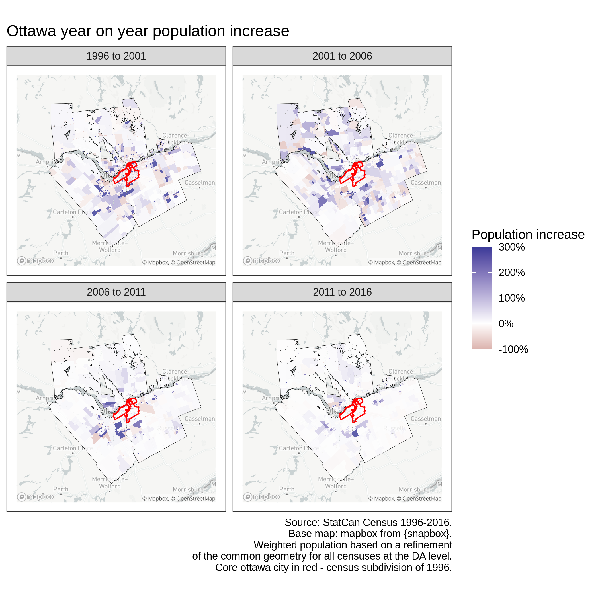
Ottwa population year-on-year growth - area weighted

Raster based

Another approach consists in using a spatial covariate that may be correlated or provide meaningful information about the variable \(v\) we are trying to interpolate. For instance, it might be useful to consider a population ecumene or other indicators of land use to perform spatial interpolation of population. Another interesting approach is to use buildings density as show in the figure below.

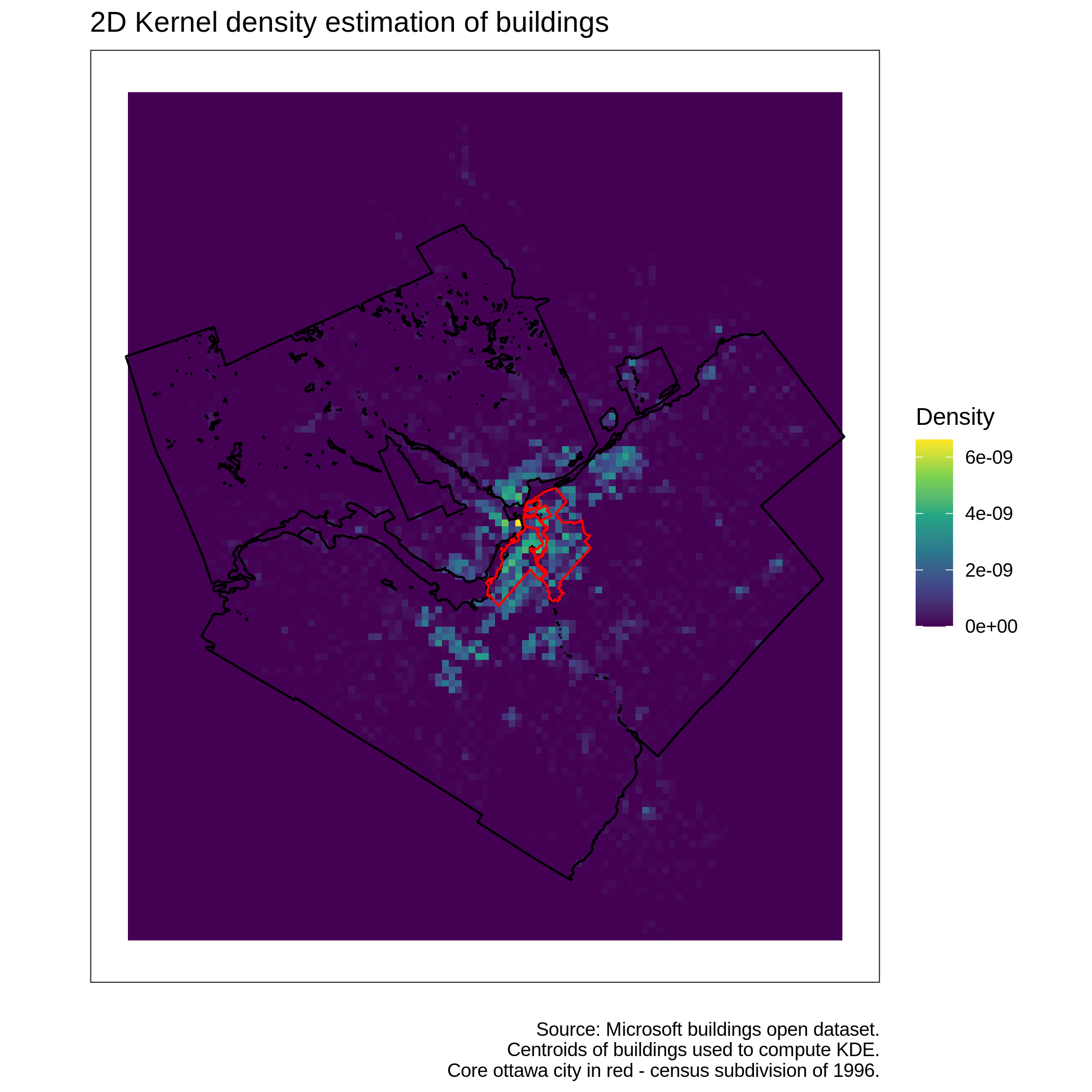
Ottwa buildings 2D kernel density estimation

In this case, the \(\kappa_i^c\) weight represents the average raster values after cropping the raster with the polygon \(i \in C\). This can be performed with the simple command kdeValsExtract <- raster::extract(rastKde, shp , fun=mean) where rastKde is a raster object representing the 2D KDE computed from the centroids of an sf buildings dataset and shp is a unique simple feature/row from the intersected sf polygon object.

This leads to the following figure, which seems qualitatively rather different from the one obtained by interpolating with polygon area. There seems to be much more areas with strong growth than previously.

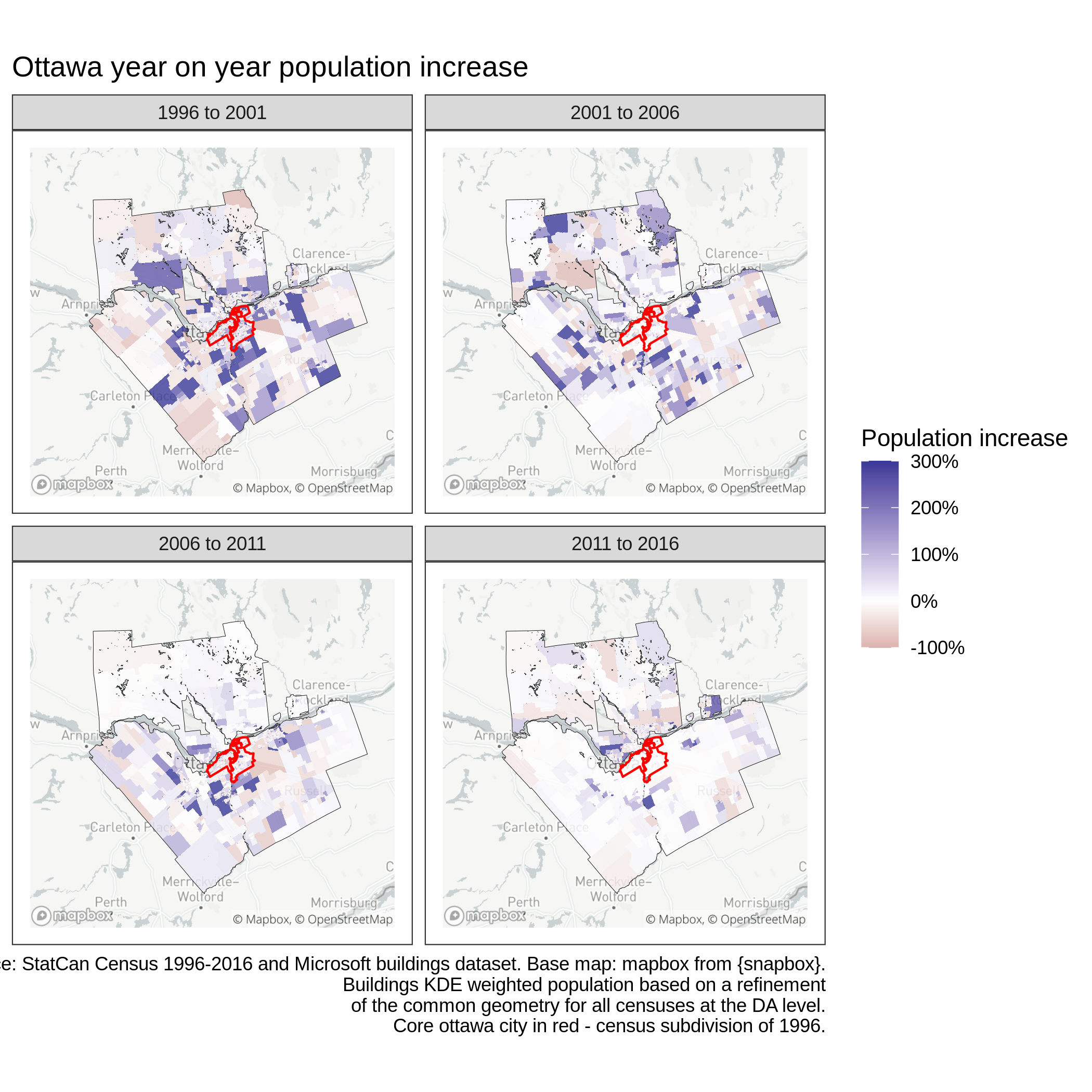
Ottwa population year-on-year growth - raster weighted

Zooming in on certain regions in the figure below however reveals that the approach is imperfect. Indeed, the weight \(\kappa_i^c\) is often close to a constant so that \(w_j^c = |N(p_a(i)|)|^{-1}, \forall j \in N(p_a(i)), \forall i \in C\). In other words, all subgeometries associated with a given polygon in the source layer \(a\) have the same weight. This can be seen in the figure below, where all polygons receive similar weight, even the small slivers with very few buildings.

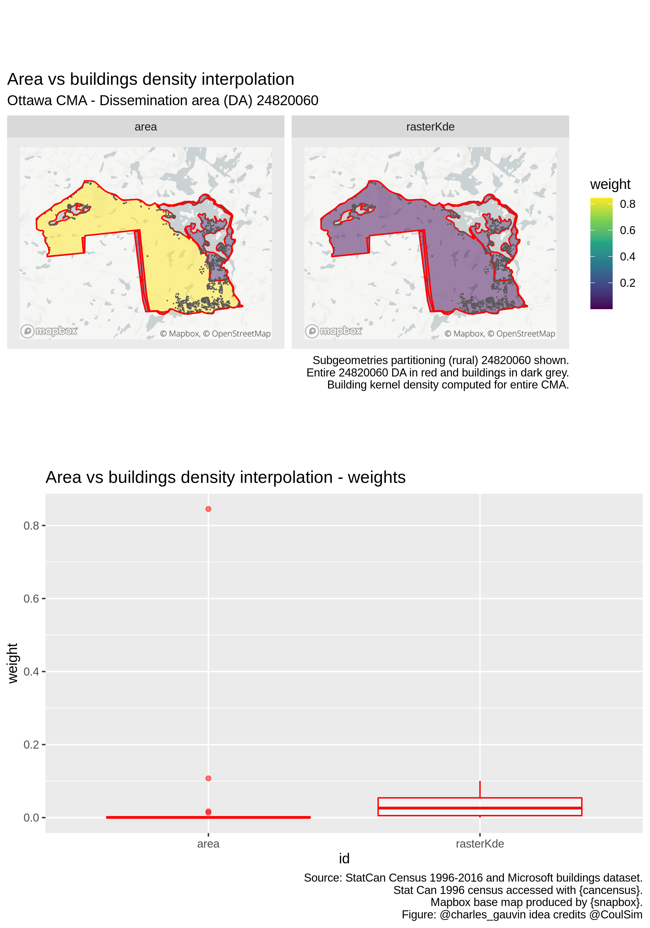
This can be explained by the fact that the KDE is computed for the entire (large) region. In addition since the function is smooth, it will have similar values for neighbouring cells. It follows that neighbouring polygons in the intersected layer will all have similar weight.

Buildings based

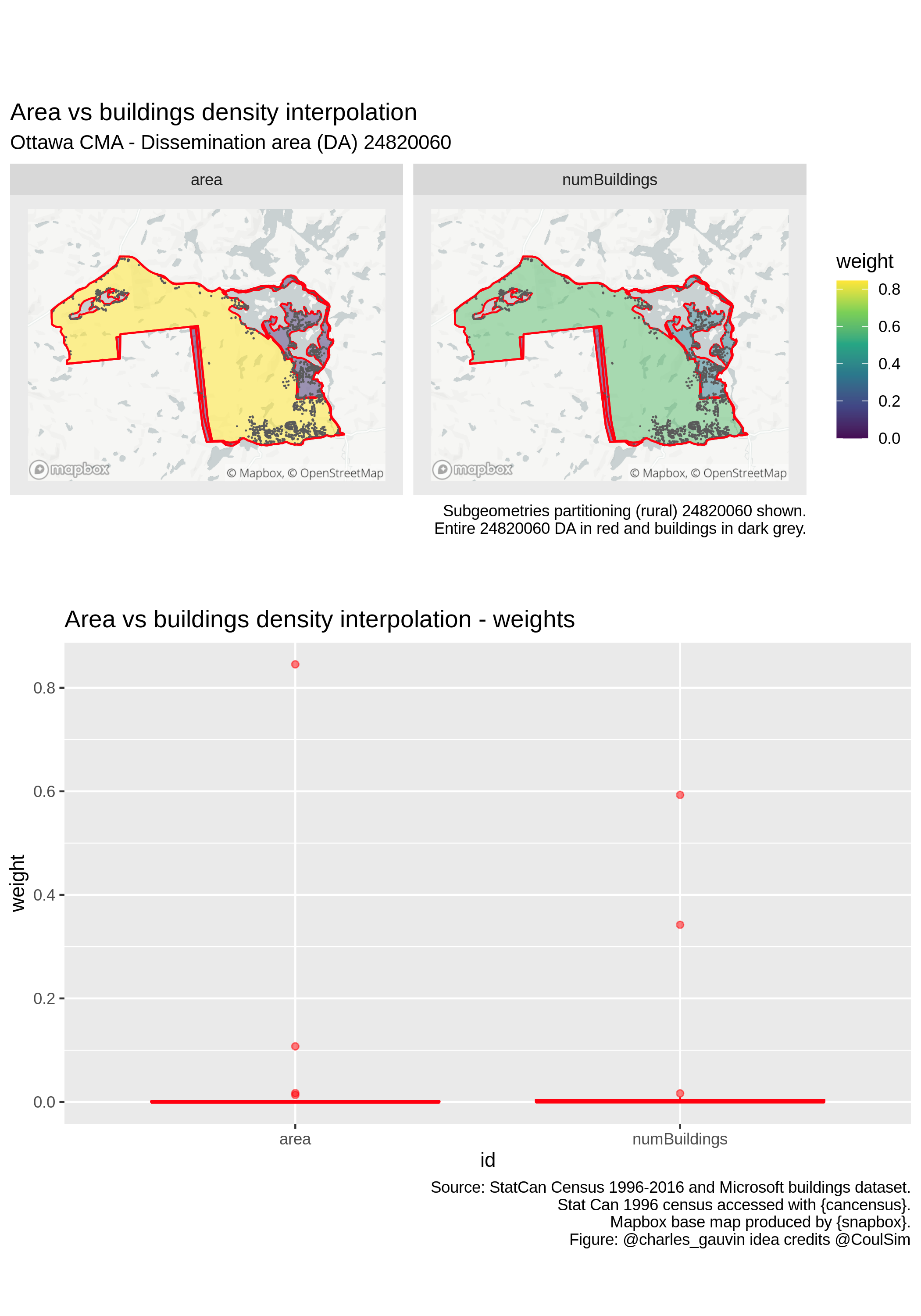
A preferable approach when trying to interpolate population might be to consider the raw number of buildings falling within each polygon \(i \in C\). Using this strategy leads to the following map, where large changes seem much more localized than with the global KDE raster weights.

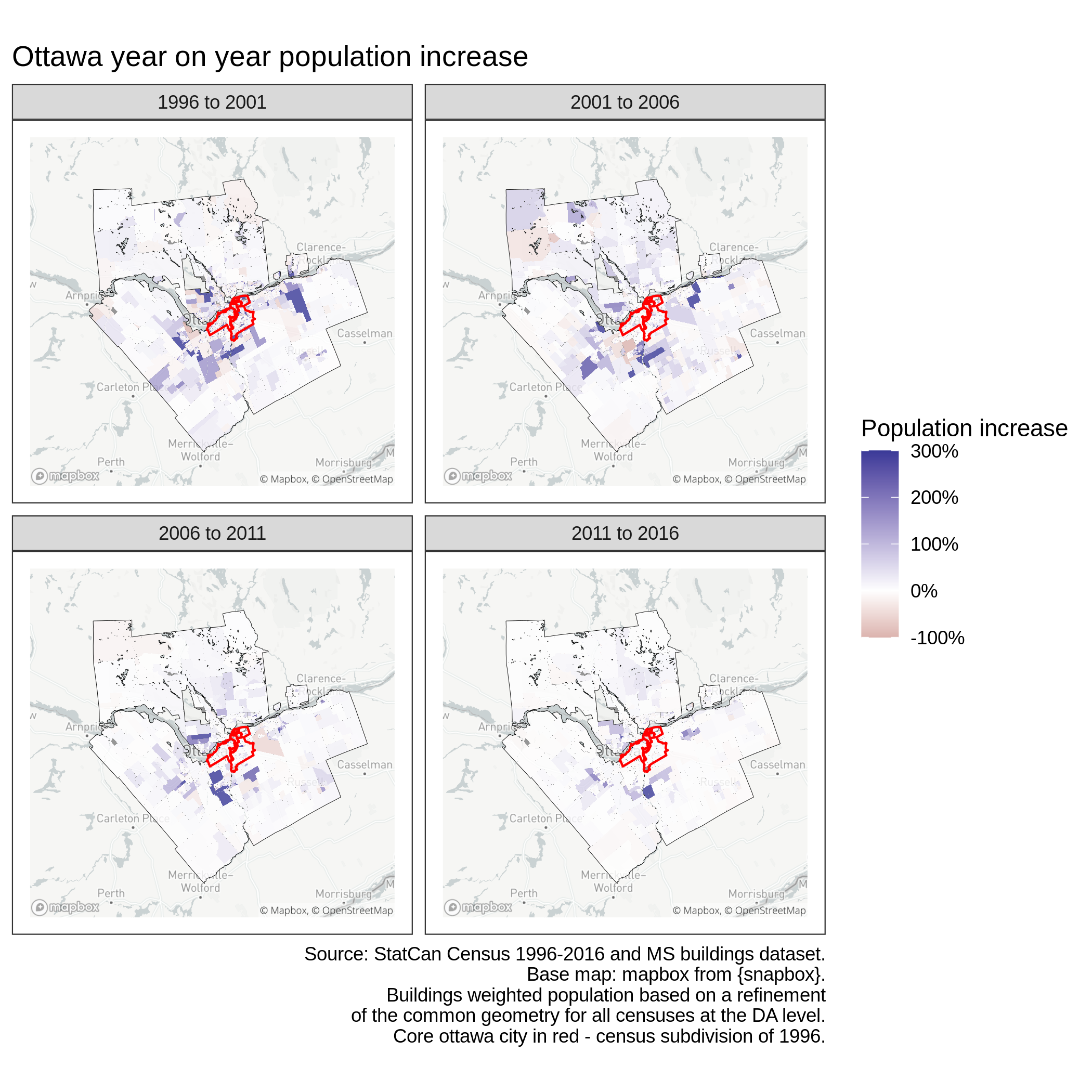
Ottwa population year-on-year growth - number of buildings weighted

As the figure below illustrates, this results in arguably better weighting for population interpolation. Indeed, considering buildings seems to correct the excessive weight of the area-based interpolation for the much larger and sparser region

Ottwa population year-on-year growth - number of buildings weighted

This is implemented very easily by a spatial join st_join(shp, shpBuildings) followed by a count of buildings by shp id. This implies that buildings that touch multiple geometries will be counted more than once. However, each building may only be counted once for each individual geometry.

Caveats

The precision of any spatial interpolation strategy crucially depends on the quality and availability of the associated covariate used to compute polygon weights. Area is a robust metric that should always be available. This is not necessarily the case of buildings. Nonetheless the Microsoft buildings dataset used for the numerical experimens is of very high quality, with close to 250 000 unique buildings for the Ottawa CMA. Comparing these figures to other authoritative datasets such as the ones computed from lidar data by various Canadian cities also confirms its excellent quality.

On the other hand, these buildings were automatically extracted with a convolutional neural network from satellite images taken at a given date, which is not precisely known.⁴ Using data that may have been captured in 2020 to perform interpolation on the 1996 census dataset is obviously questionable.

Another limitation of the approach presented above is that both the KDE and raw number of buildings counts are based on unique buildings centroids. As such, they do not consider population and a 100 floor skyscraper has the same impact as a small cabin in the woods.

Existing implementations

Although interesting, the approaches described above are simplistic and not extremely robust. There alreay exists better R implementations as well as dedicated packages to perform spatial interpolation. Functions like st_interpolate_aw from the sf package readily implements area-based interpolation while aw_interpolate from the areal package further extend the functionality.

Alternatives to spatial interpolation

Another interesting approach to deal with different incongruent geometries is to aggregate them so as to find a common tiling, which corresponds to finding connected components in the tripartite graph above. If the union of all polygons is the same for both layers, then it is always possible to do so and in the worst case we end up with a single unique geometry. This offers the important advantage of providing exact rather than approximate results, albeit on large geometries.

However, small incongruities often imply that many polygons must be aggregated into very large units, which may make it hard to provide any valuable analysis. One way to circumvent the problem for the Canadian census is to use correspondance tables provided by Statistics Canada. This approach along with more sophisticated generalizations are implemented in the tongfen package.⁵