
Distances and outlier detection
Introduction
When dealing with real datasets, which are often noisy, it is often necessary to apply outlier detection methods before carrying out any modeling or analysis. One of the simplest non-parametric methods for outlier detection is based on the Mahalanobis distance. This post shows that this distance is powerful, since it automatically identifies correlations and scales the data accordingly. It also explores its deep connection with principal component analysis (PCA) and other distances.
The Mahalanobis distance
We let \(X \in \mathbb{R}^{n\times p}\) represent our dataset where \(n\) is the number of observations and \(p\) the number of variables (we consider \(p=2\) in this example for simplicity) and we assume without loss of generality that \(X\) has zero mean. After defining the empirical covariance matrix as \(\Sigma= \frac{1}{n} X^{\top}X\),1 we obtain the (squared) Mahalanobis distance:2
\[d(x,x)^2 = x^{\top} \Sigma^{-1 } x >0.\]
As we show below, this distance is essentially the squared Euclidean distance \(d(x,x)^2 = x^{\top}x\) under a linear transformation \(\Sigma^{-1/2}\) since \(x^{\top} \Sigma^{-T/2 } \Sigma^{-1/2 } x = ||\Sigma^{-1/2 } x||_2^2\).
We can use this distance for outlier detection by removing values \(x\) from our dataset if \(x^{\top} \Sigma^{-1 } x > q\), where \(q\) is some threshold, for instance a quantile of a \(\chi^2(p)\) distribution with \(p\) degrees of freedom (more on this later).
A toy example
We start by showing some of the benefits of using the Mahalanobis compared with other distance-based alternatives for outlier detection.
Data generation
In order to build our dataset, we take 2 independent normals \(N_1\sim\mathcal{N}( 10,1^2)\) and \(N_2\sim\mathcal{N}( 3,5^2)\) and apply a (linear) rotation \(K=\frac{1}{\sqrt{2}}\begin{pmatrix} 1 & 1 \\ -1 &1 \end{pmatrix}\) so that the resulting vector \(N'=K (N_1,N_2)^{\top}\) has correlated components:
#Create the rotation matrix
mat_rot <- matrix( c(1,1,-1,1),nrow = 2,byrow = T)* sqrt(2)**-1

#Sample from the normal distributions
num_obs <- 500
mu_1 <- 10
mu_2 <- 3

sigma_1 <- 1
sigma_2 <- 5 #25 times more variance in the second dimension

norm_1 <- rnorm(n=num_obs,mu_1,sigma_1)
norm_2 <- rnorm(n=num_obs,mu_2,sigma_2)

# Rotate the generated data
norm_trans <- mat_rot %*% c(mu_1,mu_2)

norm_corr <- matrix( c(norm_1,norm_2), ncol = 2, byrow = F) %*% t(mat_rot ) #correlated data

data_corr <- data.frame( norm_corr)
data_corr$type <- 'regular'
Next, we add some outliers that follow a different cross pattern.3
# Add some outlier data that may not seem problematic if only considering the 2 dimensions in isolation

# Form a cross - add horizontal line through the mean
df_new <-  data.frame(X1= seq (min(data_corr$X1) , max(data_corr$X1) ,length.out = 10),
                      X2= rep(norm_trans[2],10))
df_new$type <- 'outlier'
data_corr <- rbind( data_corr, df_new)

# Form a cross - add vertical line through the mean
df_new <-  data.frame(X1= rep(norm_trans[1],10),
                      X2=seq (min(data_corr$X2) , max(data_corr$X2) ,length.out = 10))

df_new$type <- 'outlier'
data_corr <- rbind( data_corr, df_new)

# Form diagonal crosses by rotating the data - don't forget to center first
df_new <- df_new %>% select(X1,X2) %>% mutate( X1=X1-norm_trans[1], X2=X2-norm_trans[2]) %>% as.matrix %*% mat_rot %>% as.data.frame() %>% set_names(c('X1','X2'))
df_new %<>% mutate( X1=X1+norm_trans[1], X2=X2+norm_trans[2])
df_new$type <- 'outlier'

data_corr <- rbind( data_corr, df_new)

#Finally, center the data
data <- data_corr %>% mutate_at(vars(X1,X2), ~ scale(.x ) )
data_numeric <- data %>% select(X1,X2)
mat_data <- data_numeric %>% as.matrix
This results in the following dataset:

Outlier detection
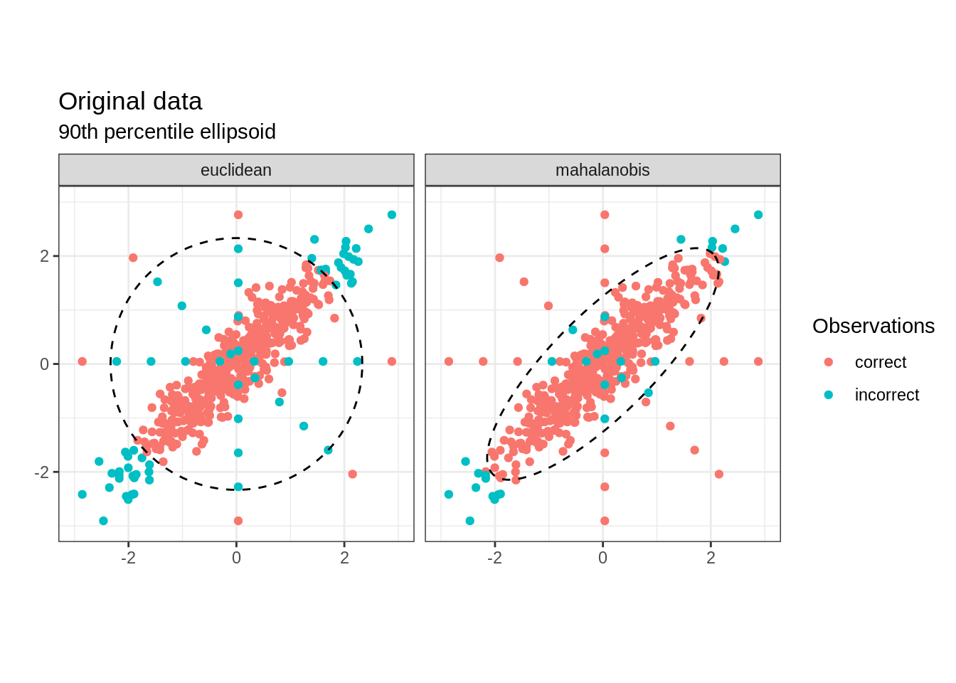
We then label observation \(x\in\mathbb{R}^{p}\) as an outlier when \(x^{\top}x > k\) or \(x^{\top}\Sigma^{-1}x > k'\), where \(k\) and \(k'\) represent the (arbitrarily chosen) \(90^{th}\) percentiles for each squared distance. On the other hand, data that lies within the ellipsoids \(\{x: x^{\top}x \leq k\}\) or \(\{ x: x^{\top}\Sigma^{-1}x \leq k'\}\) (shown in dotted lines below) is not flagged as abnormal. 4
The following plot reveals the Mahalanobis distance correctly identifies almost all true outliers, while the standard Euclidean distance fails to identify many. The Mahalanobis distance also produces a smaller number of false negative than the later. This superior performance is due to the fact that while both methods consider an ellipsoid around the mean, the Mahalanobis distance produces an asymmetrical shape that factors in the correlation in the data while the Euclidean distance creates an inaptly symmetrical region.
Mahalanobis distance and PCA
In order to understand the behaviour of the Mahalanobis distance, it is useful to study the strong relationship it shares with principal component analysis.
We can show that considering the Mahalanobis distance in the original data space is equivalent to considering the Euclidean distance in the rotated and scaled space, where the rotation and scaling are given by the eigenvectors and eigenvalues of the covariance matrix.
More specifically, since \(\Sigma\) is a square, real and symmetric matrix, we know we can compute its spectral decomposition to obtain:
\[ \Sigma= U \Lambda U^{\top} \text{ and } \Sigma^{-1}= U \Lambda^{-1} U^{\top} \]
where \(U \in \mathbb{R}^{p\times p}\) is a unitary matrix composed of the eigenvector of \(\Sigma\) such that \(UU^{\top}=U^{\top}U=I\) and \(\Lambda = \text{diag}(\lambda_1,\cdots, \lambda_p)\) is a diagonal matrix formed of the eigenvalues of \(\Sigma\), where \(\min_i \lambda_i >0\).
If we set \(W=X U\), then we observe that:
\[ \begin{align} \frac{1}{n}W^{\top}W &= U ^{\top} X ^{\top}X U \\ & = U ^{\top} \Sigma U \\ & = U ^{\top} U \Lambda U^{\top} U \\ & = \Lambda \end{align} \]
and so the new dataset \(W\) we obtain by rotating the data with \(U\) is uncorrelated and the \(i^{th}\) component has variance \(\lambda_i\). This is exactly the rotatation that is obtained by applying PCA to the original data. Indeed, the following R code performs the transformation by leveraging prcomp:
# Find the rotation matrix by applying PCA OR computing the eigenvectors from the covariance matrix directly
pca_results <- prcomp(data_numeric, scale = FALSE)

#this line below should match eigen(cov_mat)$vectors (up to -1)
eig_vectors <- pca_results$rotation

#this line below should match pca_results$x
data_rotated <- data.frame (as.matrix(data_numeric)%*% eig_vectors) %>% set_names(c('X1','X2') )
We then obtain the following figure:
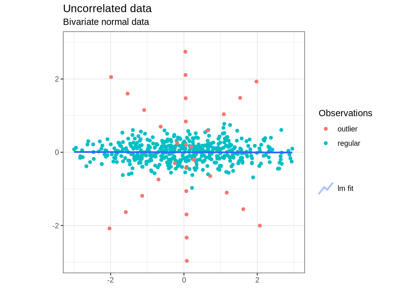
From the figure above, we notice that the first dimension is much more variable than the second (from the eigenvalues, approximately 9.5 times more variable), due to the way we generated the initial dataset.
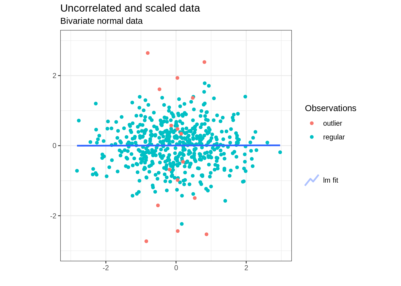
We can normalize the data by scaling by the standard deviation of each component, which is the square root of the eigenvalue. Indeed, if we let \(Z=X U \Lambda^{-1/2}\), then \(\frac{1}{n} Z^{\top}Z =I\). It also follows we can write \(\Sigma^{-1} = \Sigma^{-T/2} \Sigma^{-1/2}\) by taking \(\Sigma^{-1/2}=\Lambda^{-1/2} U^{\top}\) and so, as promised in the introduction, we have \(x^{\top} \Sigma^{-T/2 } \Sigma^{-1/2 } x = ||\Sigma^{-1/2 } x||_2^2\).
This scaling is easily performed with the following code:
# pca_results$sdev**2 should give the same results as eigen(cov_mat)$values
eig_values <- pca_results$sdev**2

# Scale the rotated data with the eigenvalue
#remember,the eigenvalues correspond to the variance of the rotated variables
#we want to scale by the std dev=var**0.5
data_rotated_scaled <- data.frame (as.matrix(data_rotated)%*% diag(eig_values**-0.5)) %>% set_names(c('X1','X2') )
and we obtain the following symmetrical dataset:
How is this transformation related to the Mahalanobis distance? In fact computing the Euclidean distance in the new rotated and scaled space shown above is exactly equivalent to computing the Mahalanobis distance in the original data space:
With \(z_i=\Lambda^{-1/2} U^{\top} x_i\):
\[ \begin{align} z_i^{\top}z_i &= z_i^{\top}U \Lambda^{-1/2} \Lambda^{-1/2}U^{\top}z_i \\ &= x_i^{\top}\Sigma^{-1}x_i. \end{align} \]
In fact, the elongated ellipsoid in the second figure in this post was computed using this identity. This is illustrated in the code below where we first compute the Euclidean distance in the scaled and rotated space and identify the outliers using the \(90^{th}\) percentile.
#Euclidean Norm
norm_2_fun <- function(x){
  sqrt(sum(x**2))
}

#Compute the norm for all observations
dist_rotated_scaled <- data.frame(dist= map_dbl(1:nrow(data_rotated_scaled),
                                          ~norm_2_fun(data_rotated_scaled[.x, ]-mean_scaled))
)

#Get the 90th percentile in the rotated and scaled space using the Euclidean Distance
quant_original_outlier <- quantile(dist_rotated_scaled$dist, probs = 0.9)
Next, we take a unit circle and apply the appropriate inverse transformation to get back the ellipsoid in the original data space:
#unit circle in the scaled and rotated space
unit_circle <- map_dfr(seq(0,2*pi,by=pi/64),
                       ~ data.frame(cos(.x),sin(.x))) %>% set_names(c('X1','X2'))

#mahalanobis ellipsoid in original space
#{x: ||Lambda**-0.5 U' (x-x_0)' ||_2 \leq r} = {x: x=  sqrt(r) U Lambda**0.5 *B + x_0}, where x_0 is the mean and B is the unit Ball
mahalanobis_orig_space <- data.frame(as.matrix(unit_circle * sqrt( quant_original_outlier ) ) %*% diag(eig_values**0.5) %*% t(eig_vectors))
Instead of considering a simple quantile based on the data. It could have been appropriate to consider a priori the \(90^{th}\) quantile of a \(\chi^2(p)\) distribution with \(p\) degrees of freedom. Indeed, Since our original data \(X\) is multivariate normal, then so is the rotated and scaled \(Z\). Moreover, \(z_1\) and \(z_2\) are orthogonal due to the rotation. They also both have variance 1 due to the scaling. It follows that \(z_1^{\top}z_2 \sim \chi^2(p)\) and hence \(\chi^2(p)^{-1}(0.9)\) would be a good candidate threshold for outlier detection.
Mahalanobis and Euclidean distance
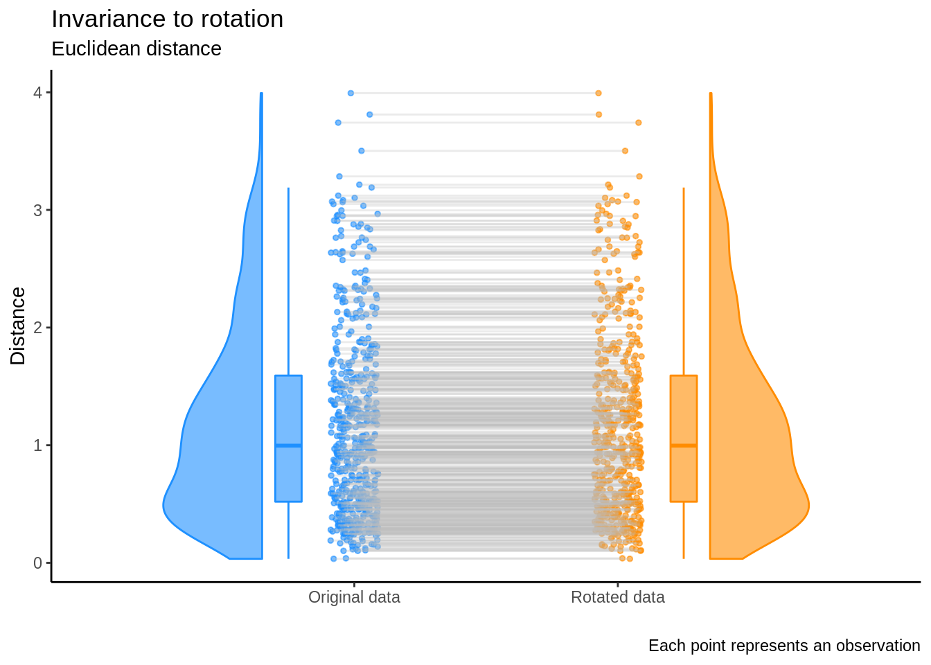
In this final section, we compare the relationships between the different distances we’ve considered. First, it it important to note that applying a rotation on the dataset does not change the norm of any observation. Indeed, if \(w_i=U^{\top}x_i\), then: 5:
\[ \begin{align} w_i^{\top}w_i &= x_i^{\top}UU^{\top}x_i \\ &= x_i^{\top}x_i \end{align} \]
This shows that the Euclidean norm is invariant under rotation and is visually illustrated in the plot below:
On the other hand, we’ve also seen that if \(Z=X U \Lambda^{-1/2}\), then
\[ \begin{align} z_i^{\top}z_i &= x_i^{\top}U \Lambda^{-1/2} \Lambda^{-1/2}U^{\top}x_i \\ & = x_i^{\top}\Sigma^{-1}x_i \\ & \neq x_i^{\top} x_i, \quad \text{ if } x \neq 0 \end{align} \]
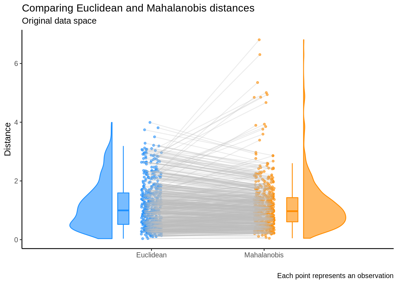
and so the Euclidean distance is not invariant under the linear transformation \(U \Lambda^{-1/2}\). This also implies that results will differ when comparing the standard Euclidean distance and the Mahalanobis distance in the original data space. The rain plot below illustrates this discrepancy by showing the change in rank when comparing \(x_i^{\top} x_i\) and \(x_i^{\top}\Sigma^{-1}x_i\). 6
Conclusion
We’ve seen that the Mahalanobis distance is the Euclidean distance under a specific linear transformation.
This distance is efficient because it implicitly rotates and scales the data based on the eigenvector and eigenvalues of the covariance matrix. This rotation is exactly the same as the one performed by principal component analysis to identify the orthogonal components in the data.
In the ideal situation where the data really follows a multivariate normal distribution, this transformation leads to independent standard normal random variables whose sum of squares follows a chi square distribution.
Scaling by \(\frac{1}{n-1}\) or any other constant would not change the analysis presented here. The important assumption is that \(\Sigma\) is real and symmetric.↩
In fact, we can induce similar distances with any real semi-definite positive matrix \(\Gamma\) for which the following decomposition exists \(\Gamma=\Gamma^{T/2}\Gamma^{1/2}\). In that case, we have \(||x||_{\Gamma} = ||\Gamma^{1/2}x||_2 = \sqrt{x^{\top} \Gamma^{T/2} \Gamma^{1/2} x} >0\).↩
These new points would not necessarily be flagged as outliers if considering each dimensions independently, since they lie within the box \([\underline{x}_1, \bar{x}_1] \times [\underline{x}_2, \bar{x}_2]\), where each elements represent the min and max over each dimension for the valid non-outlier data.↩
The transpose is not an error, \(w_i\in \mathbb{R}^{p}\) and \(x_i\in \mathbb{R}^{p}\) are column vectors and correspond to rows in \(W\in \mathbb{R}^{n\times p}\) and \(U\in \mathbb{R}^{n\times p}\), respectively.↩
This plot corresponds to the distance between each of the data points and the mean of the original data (which is 0) since \(x_i^{\top} x_i=(x_i-0)^{\top} (x_i-0)\). Taking distances with respect to another point \(x_0\) yields the same ordering and \((x_i-x_0)^{\top}(x_i-x_0) \neq (x_i-x_0)^{\top}\Sigma^{-1}(x_i-x_0)\) if \(x_i \neq x_0\).↩
