Notation

We define the set of real symmetric positive definite \(n\) dimensional matrices as \(\mathbb{S}_{++}^n\). This is the set of matrices \(X\in \mathbb{R}^{n \times n}\) such that \(u^{\top}Xu >0 , \forall u \neq 0\) and \(X=X^{\top}\). We can assume without loss of generality that \(X\) is full rank, since we could remove colinear rows and columns and we are only interested in non-degenerate ellipsoids. \(\mathcal{B}_n = \{ u \in \mathbb{R}^n: ||u||\leq 1\}\) represents the unit ball in \(\mathbb{R}^n\) and \(||u|| = (u^{\top}u)^{1/2}\) is the regular Euclidean 2-norm.

Ellipsoids as affine transformations of the unit ball

An ellipsoid is an affine transformation of the unit ball. Using the Choleksi decomposition, we have:

\[ \begin{align} \mathcal{E} &= \{u: (u-c)^{\top} X (u-c) \leq 1 \} \\ &= \{u: (L^{\top}(u-c))^{\top} (L^{\top}(u-c)) \leq 1 \} \\ & = \{L^{-\top}a + c: ||a||_2 \leq 1 \} \\ & = L^{-\top} \mathcal{B}_n+ c \end{align} \]

where and \(L^{\top}\) is lower triangular. For some matrix \(X \in \mathbb{S}_{++}^k\), the decomposition \(X=LL^{\top}\) is unique. Since \(det(X) = det(L)^2\), we note that \(det(X) > 0\) and \(det(L)>0\) if \(X\) is full rank.

A real symmetric matrix can be diagonalized using the spectral decomposition \(X= U\Lambda U^{\top}\) for some diagonal \(\Lambda\) and unitary matrix \(U\). It follows that we can express any ellipsoid as:

\[ \begin{align} \mathcal{E} &= \{u: (u-c))^{\top} U \Lambda U^{\top} (u-c) \leq 1 \} \\ & = \{u: (\Lambda^{1/2} U^{\top} (u-c))^{\top} (\Lambda^{1/2} U^{\top}(u-c)) \leq 1 \} \\ & = U^{-\top} \Lambda^{-1/2} \mathcal{B}_n+ c \end{align} \]

It also follows that in this case all eigenvalues must be positive since \(det(X) = det(\Lambda) = \Pi_{i=1}^n \lambda_i\).

For any \(X \in \mathbb{S}_{++}^k\), we can also show that there exists a unique \(A \in \mathbb{S}_{++}^n\) such that \(X=A^2\). Existence is easy to check by setting \(A=U\Lambda^{1/2} U^{\top}\) and is sufficient for our purposes. For more details, see these lecture notes. Using this positive definite square root, we can express the ellipsoid as:

\[ \begin{align} \mathcal{E} &= \{u: (u-c))^{\top} AA (u-c) \leq 1 \} \\ & = \{u: (A (u-c))^{\top} (A (u-c)) \leq 1 \} \\ & = A^{-1} \mathcal{B}_n+ c \end{align} \]

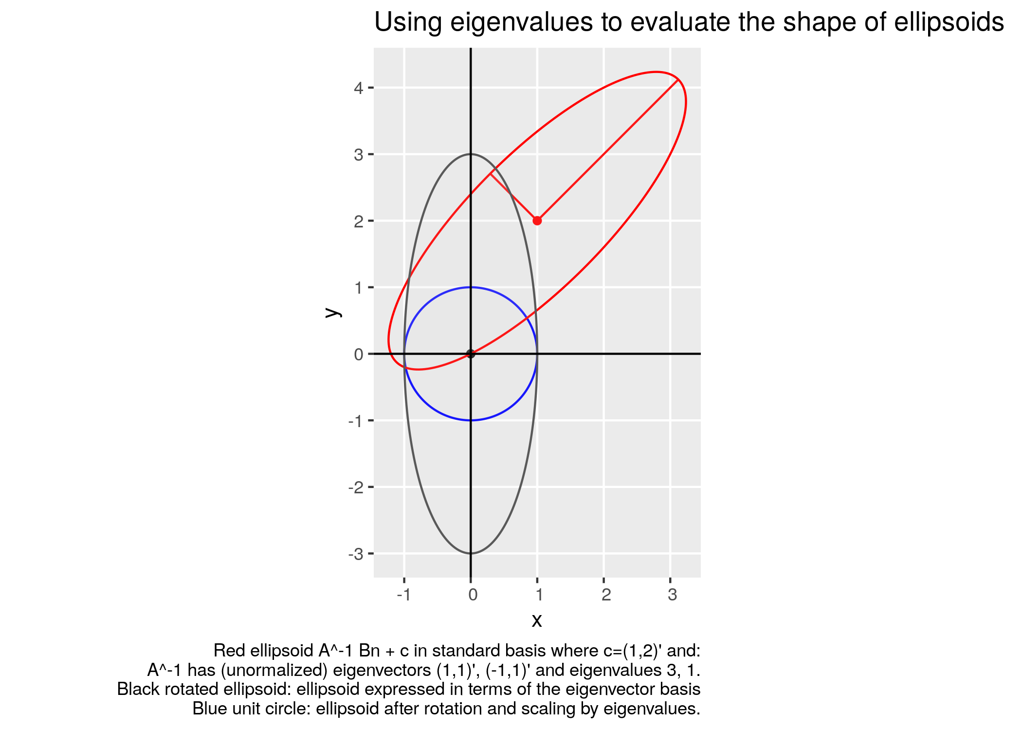
Eigenvalues

By exploiting the fact that the ellipsoid \(\mathcal{E}\) is defined by the affine transformation \(x\rightarrow A^{-1} x +c\), we can determine its elongation by comparing the ratio of the mininum and maximum eigenvalues of \(A\), which are equal to those of \(L\) and \(L^{\top}\) as well as the square root of those of \(X\).

Indeed, rotating the points \(s \in S\) using \(U\) expresses them using the orthogonal basis formed by the eigenvectors of \(X\), which are the same as those of \(A\), \(L\) and \(L^{\top}\). Comparing the ratio of eigenvalues therefore allows us to determine the relative importance of each axis. In 2 dimensions we would compare the principal and minor axis, which correspond to the width and height of the ellipsoid. The following figure helps build intuition on these transformations.

Minimum volume bounding ellipsoid (MVE)

We can also show that the volume of the ellipsoid is equal to:

\[ \begin{align} det(L^{-\top}) Vol(\mathcal{B}_n) &= det(A^{-1}) Vol(\mathcal{B}_n) \\ &= det(X^{-1})^{\frac{1}{2}} Vol(\mathcal{B}_n) \\ &= det(U^{-\top}) \Pi_{i=1}^n \lambda_i^{-1/2} Vol(\mathcal{B}_n) \\ &= \Pi_{i=1}^n \lambda_i^{-1/2} Vol(\mathcal{B}_n) \end{align} \] by noting that the determinant of the unitary matrix \(U\) is 1 (see these lecture notes for further details). We also observe that the eigenvalues of \(L\) and \(A\) are the square root of those of \(X\).

It follows that we can find the minimum volume ellipsoid that contains all points in a closed, non-empty and bounded set \(S\in\mathbb{R}^n\) by solving the following convex optimization problem¹:

\[A^{*},c^* \in \displaystyle \arg\min_{A \in \mathbb{S}_{++}^n, c} \{ -\log(\det(A)) : ||A(s-c)||_2\leq 1 , \forall s \in S \}\]

This problem is convex since it consists of minimizing \(-log (det)\), which is convex over \(\mathbb{S}_{++}^n\) (see page 74 of Boyd and Vanderberghe book) while respecting convex second order cone constraints.

For a general set \(S\), this would result in a hard semi-infinite optimization problem. Indeed, there are as many second order cone constraints as the cardinality of \(S\) and \(\max_{s \in S} ||A(s-c)||_2\) amounts to maximizing a convex quadratic function over a possibly non-convex set \(S\), which is intractable. It is therefore impossible to handle these constraints by using robust optimization techniques.

However, if \(S\) is a finite discrete set \(S=\{s_1, \cdots, s_N \}\) for some finite \(N\), we obtain a finite number of convex inequalities and we can solve the problem fairly efficiently using off-the-self interior point solvers. This problem also offers several appealing properties, which are presented next.

Invariance to taking the convex hull

It is possible to show that computing the minimum volume bounding ellipsoid on \(S\) or its convex hull is the same. Consider the following restriction of the initial problem where the second order cone constraints must hold for \(conv(S) \supseteq S\), where \(conv(S)\) represents the convex hull of \(S\) and \(\mathcal{E}^{conv(S)}\) is the ellipsoid defined by the optimal solution of the following problem:

\[A^{conv(S)*} , c^{conv(S)*} \in \displaystyle \arg\min_{A \in \mathbb{S}_{++}^n, c} \{ -\log(\det(A)) : ||A(s-c)||_2\leq 1 , \forall s \in conv(S) \}\]

If \(\mathcal{E}\) is the minimum volume bouding ellipsoid for the set \(S\), we can see that \(conv(S)\subseteq \mathcal{E}\), since \(conv(S)\) is the smallest convex set containing \(S\) and \(\mathcal{E}\) is also convex. Hence \(S \subseteq conv(S) \subseteq \mathcal{E} \subseteq \mathcal{E}^{conv(S)}\) and it follows that \(\mathcal{E}=\mathcal{E}^{conv(S)}\) since \(\mathcal{E}^{conv(S)}\) must have minimal volume over all bounding ellipsoids and the Löwner-John theorem asserts that this minimal ellipsoid is unique.

As the case study below highlights, this simple property can lead to sizeable computational speedups since it can considerably reduce the number of constraints.

Invariance to shift and scaling

The fact that the ellipsoid is defined by an affine mapping offers the advantage that the eigenratios are invariant to shifts and scaling. Indeed, the minimum volume bounding ellipsoid for the set \(\alpha S + \beta\) for arbitrary \(\alpha >0 , \beta \in \mathbb{R}\) is simply the minimum volume bounding ellipsoid for \(S\) scaled by \(\alpha\) and shifted by some offset².

This namely implies that it is immaterial wether we apply scaling transformations such as \(s \rightarrow (s-s_{min})/(s_{max}-s_{min})\), where \(s_{min} = \min_{s \in S} s\) and \(s_{min} = \max_{s \in S} s\). In practice however, specific coordinate reference systems (crs) with large offsets expressed in meters can lead to numerical issues and it is therefore preferable to scale the coordinates.

Overview

We consider a practical context where shapes are given in the form of a set of discrete points. In our specific context, we have neighbourhood shapes in ESRI shapefile format for Quebec City and Montreal. These are either polygons, collections of polygons (for instance in the case of neighbourhoods with discontiguous regions such as islands) or even heterogeneous geometry collections with linestrings. To compute bounding ellipsoids over discontiguous collections of geometries, we exploit the property presented above and always consider the convex hull.

Although the method only applies straightforwardly to finite collections of points, it remains useful for most practical applications since census and other administrative boundaries often use this representation. Although we only consider the two dimensional case where dimensions represent longtitude and latitude or x and y offsets, the method can be generalized to any number of dimensions.

Using this simple methodology, we can answer questions such as: is a region more elongated than another and to what extent is a region stretched. Since \(\lambda_{max}(B)/\lambda_{min}(B) \in [1, \infty)\), any circle has minimal eigenratio while an inifintely thin ellipsoid has an infinitely large ratio.

City-wide comparisons

We begin by comparing the entire cities of Quebec City and Montreal. As mentionned in this other post, various metrics suggest that Quebec is much more circular/symmetric than Montreal. Comparing the ratio of eigenvalues for the minimum volume bounding ellipsoid of both cities confirms that this is true, Quebec has a ratio of 1.05, rather close to the lower bound of 1, while for Montreal this figure jumps up to 1.66.

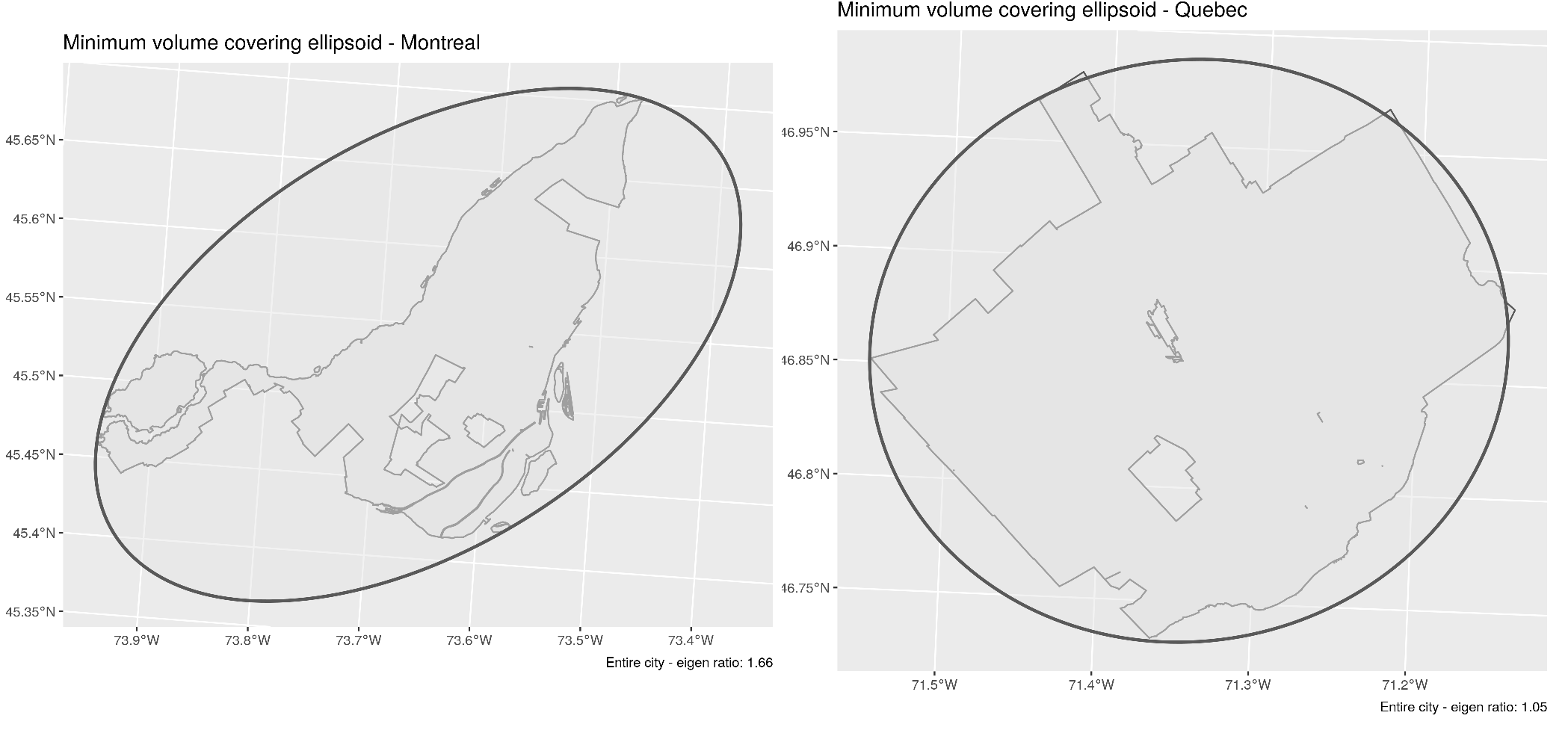
Comparing the shape of Montreal (left) and Quebec City (right)

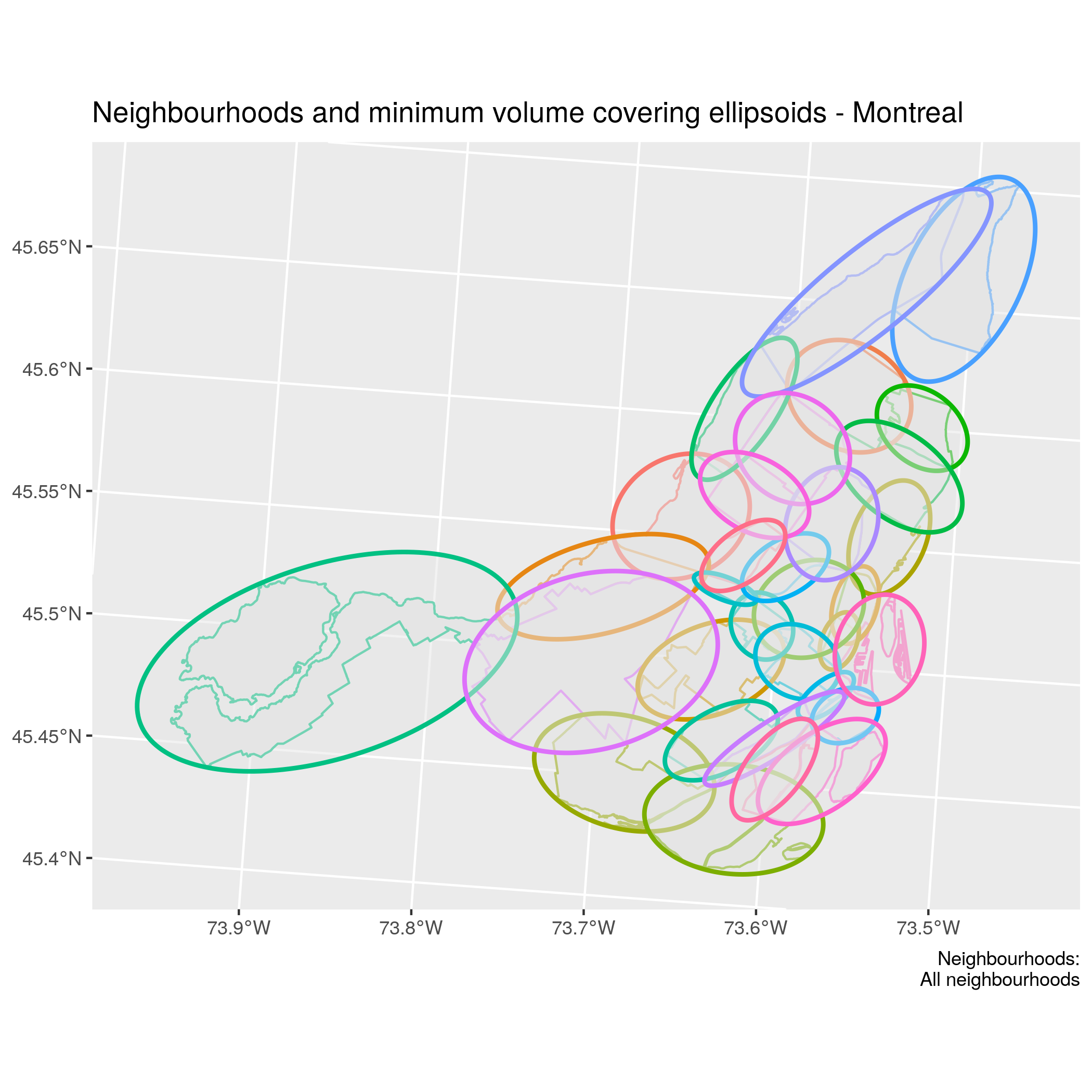
##Neighbourhood-level comparisons

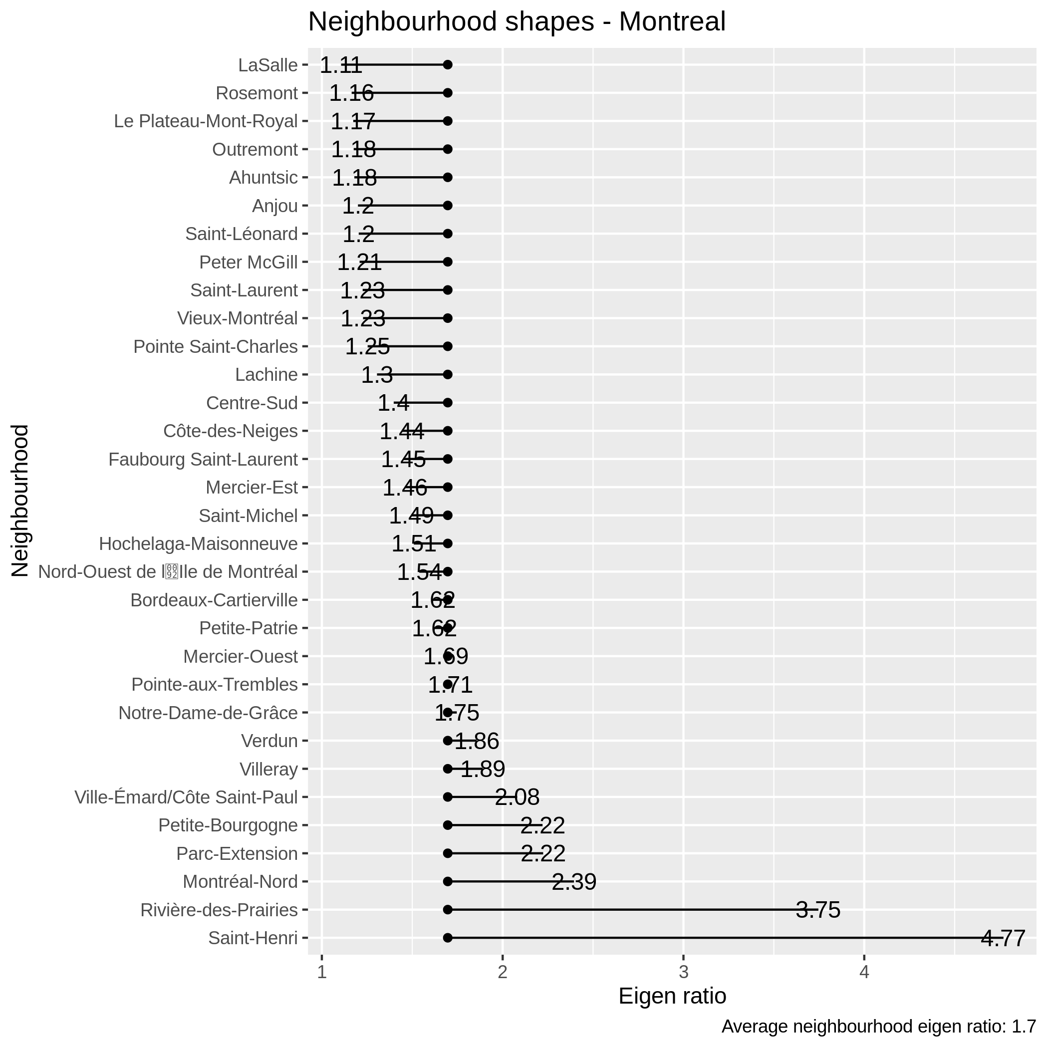
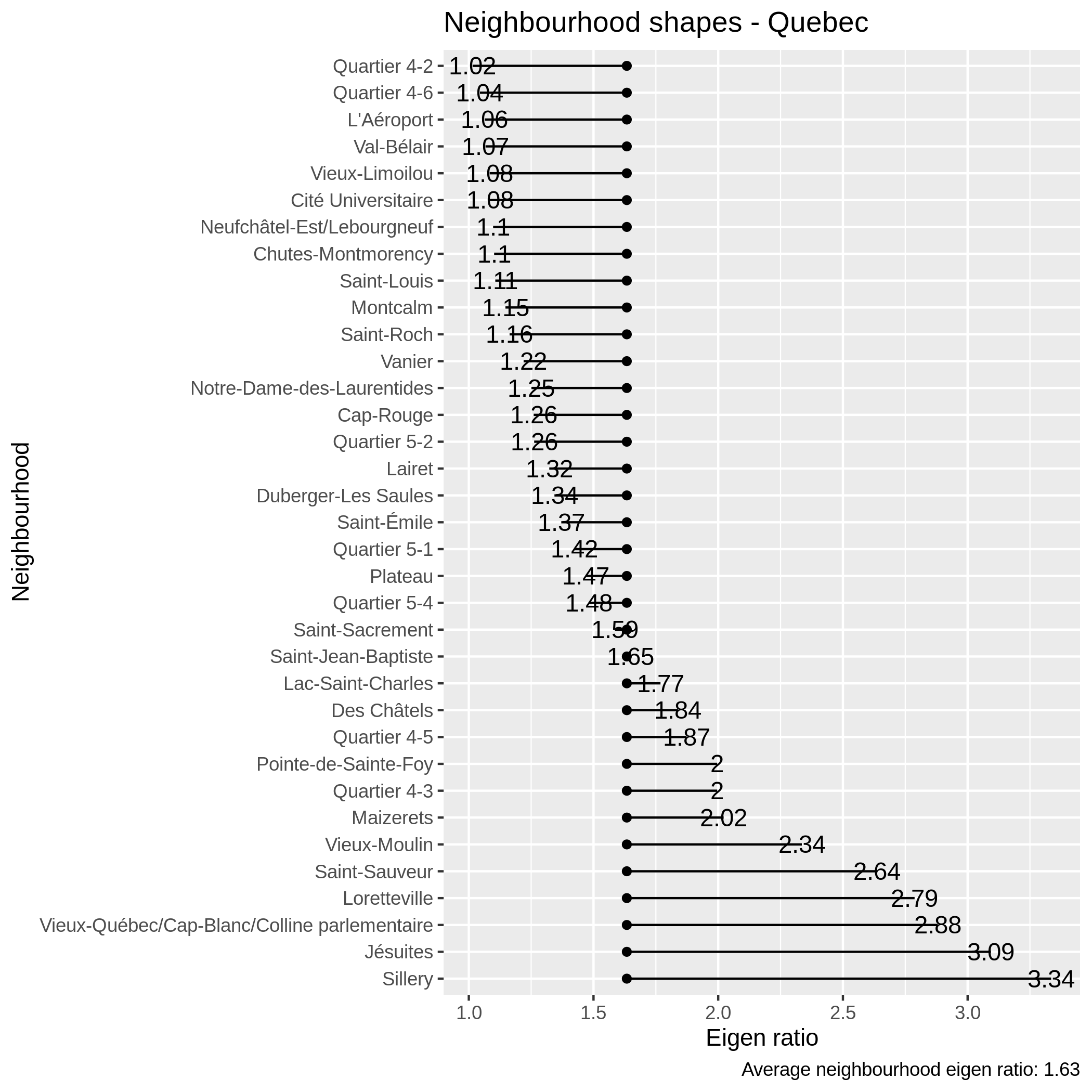
Performing the analysis for each of the 32 and 35 neighbourhoods making up Montreal and Quebec City, we obtain the following figures:

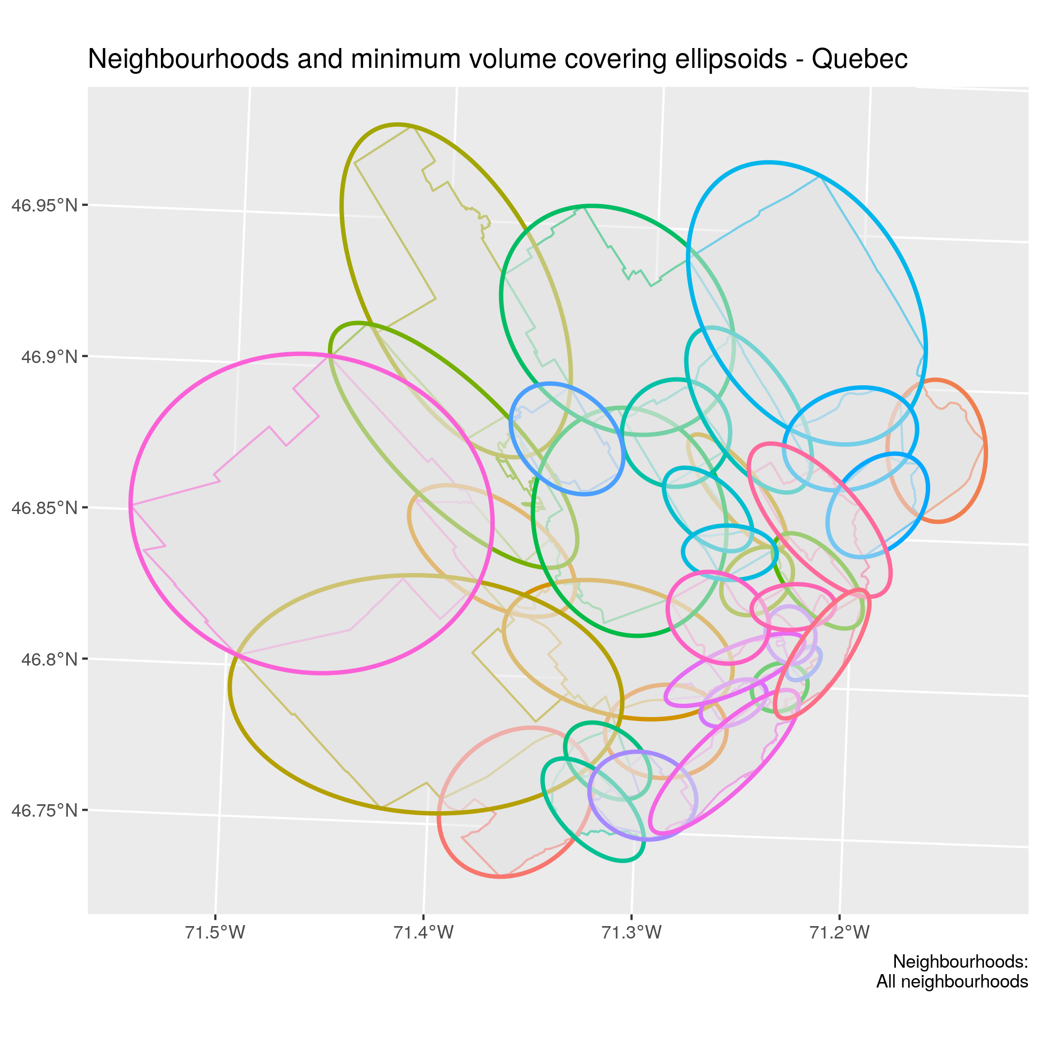
Quebec city neighbourhoods and minimum volume covering ellipsoids

Comparing the distribution of eigenratios over neighbourhood allows us to see that Montreal is also slightly more elongated at the neighbourhood level on average.

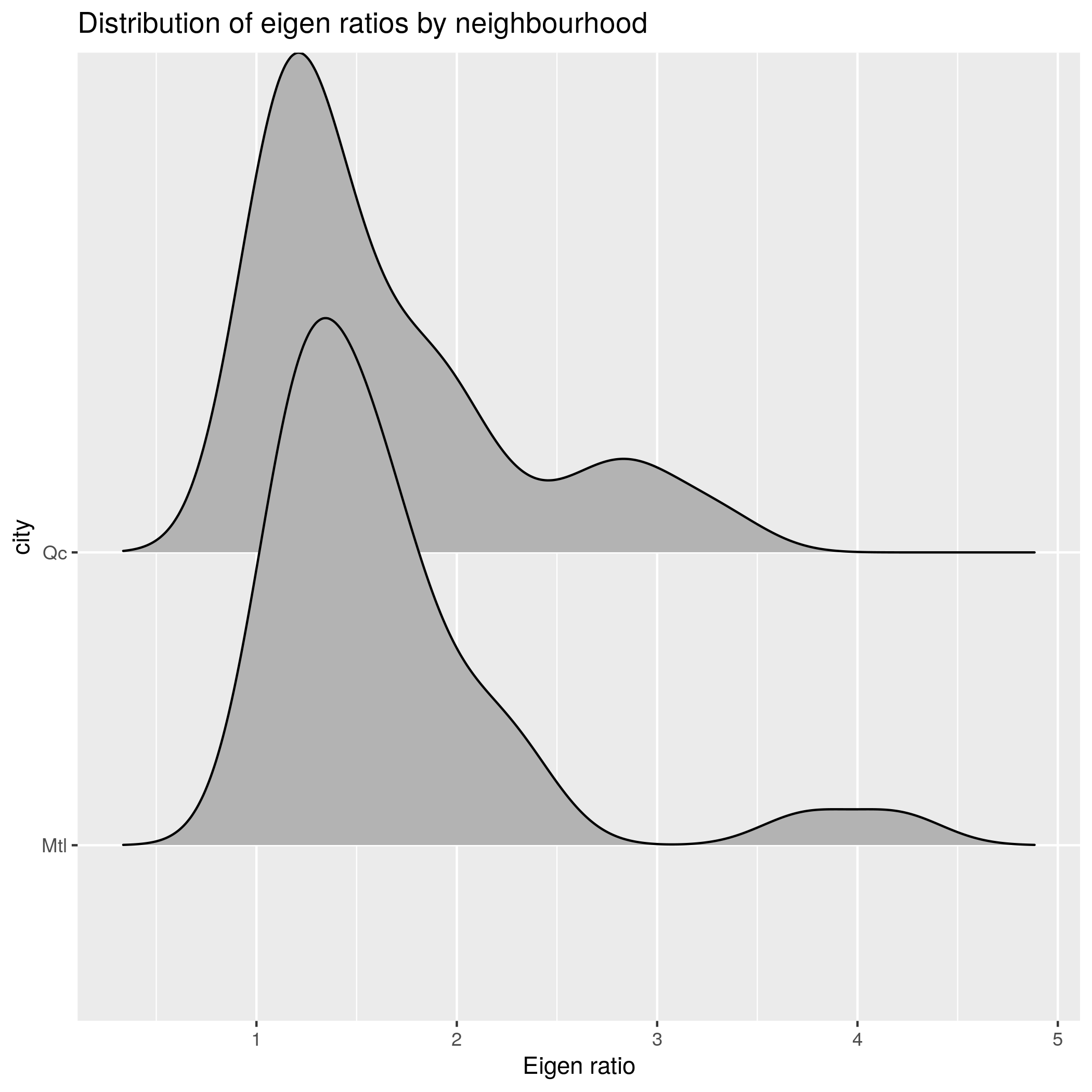
Comparing the eigenratio distribution by neighbourhood

This is mostly due to the fact that Montreal has some large elongated outliers. Saint-Henri and Rivière des prairies both have a height more than 3.5 times its width.

Comparing the eigenratio distribution by neighbourhood

Although Quebec is less variable at the neighbouhood level, it also has some relatively elongated neighbourhoods. Nonetheless, we also observe that 8 neighbourhoods in Quebec have a ratio no larger than the ratio of LaSalle, the minimal neighbourhood in Montreal.

Comparing the eigenratio distribution by neighbourhood

Quick analysis

All 3 most elongated neighbourhoods in Montreal are adjacent to a water body while for Quebec City this is true for 2 of the 3 most elongated neighbourhoods. In the case of Montreal, Saint-Henri is delimited by the canal de Lachine while Sillery is delimited by the Saint-Lawrence River.

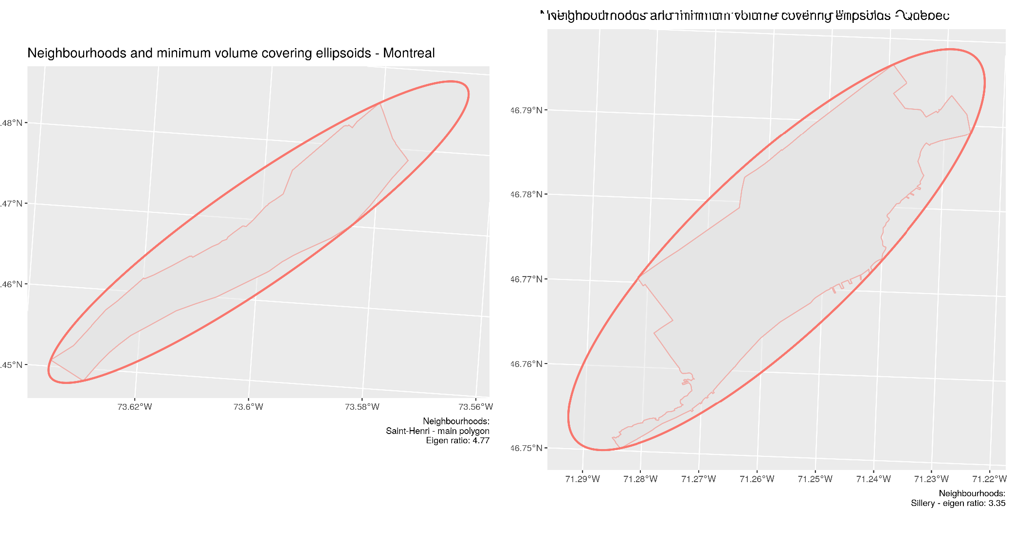
Most elongated neighbourhoods for Montreal: Saint-Henri (left) and Quebec City - Sillery (right)

The neighbourhoods with the smallest eigenratios have remarkably symmetric distribution. Quartier 4-1 in Beauport, Quebec is almost a perfect square. It seems probable that various neighbourhoods without any clear natural or sociological delimitations could have more symmetric shapes. This might namely be the case for more recently developped suburbs with few natural constraints. For Quebec City at least, this seems to be somewhat corroborated. However, various factors can influence the shape of neighbourhoods.

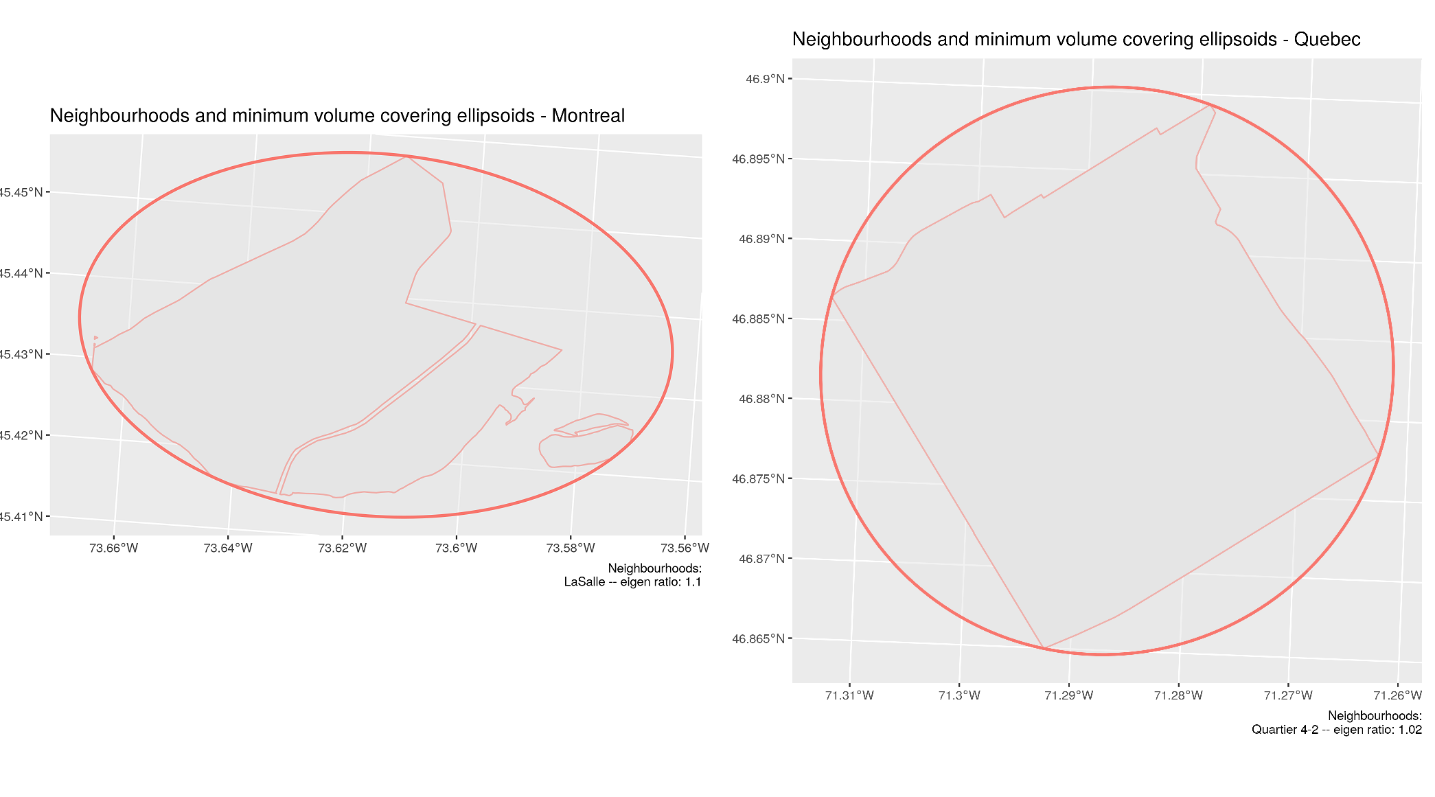
Most symmetric neighbourhoods for Montreal: LaSalle (left) and Quebec City - Quartier 4-1 (right)

Computational performance

Using the raw set of points \(S\) defining each region, solving the problem took from a 6.3 seconds to a 6.9 minutes with sets of 64 to 2865 points. However, as the following graph illustrates, using the convex hull produced remarkable speedups. Indeed, particularly for irregular geometries, the convex hull is represented by much fewer points than the original shape. This reduces the number of second order cone constraints and considerably helps reduce the speed of computing the minimum volume bounding ellipsoid. With the convex hull, problems took only from 0.9 to 44 seconds to solve.

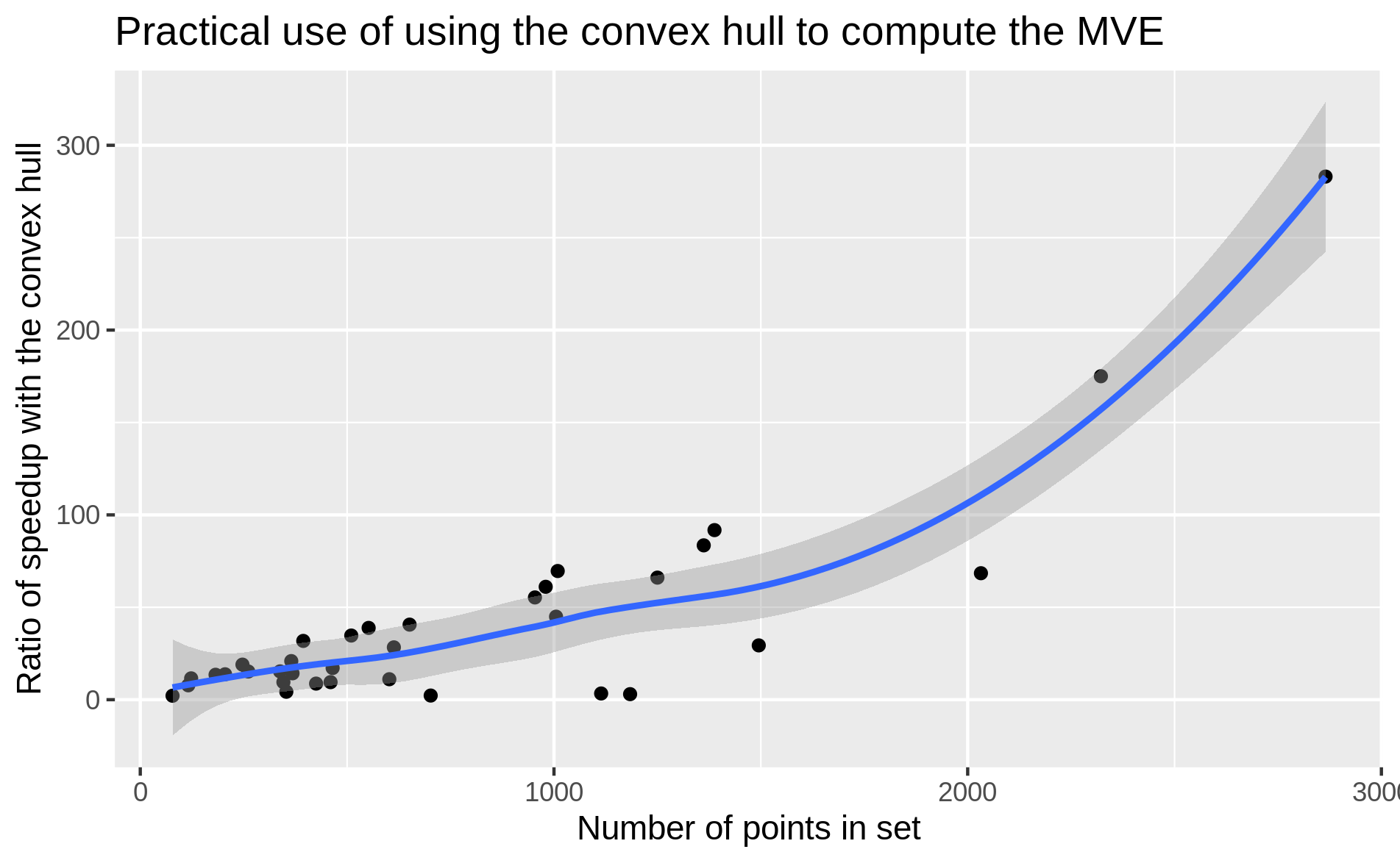
Speedup (initial time/convex hull time) achieved by using the convex hull to compute minimum volume bounding ellipsoids

For our numerical experiments, minimum volume bounding ellipsoid where obtained by modeling the problem in R with CVXR and using the ECOS solver. Using more specialized software or algorithms, could accelerate the procedure even more, which might make it applicable for large-scale problems involving thousands of regions.

Caveats

Although identifying shapes that are very elongated may prove useful to identify gerrymandered districts, the eigenratio proposed in this post has limitations. As the following figure reveals, it is possible that neighbourhoods have very irregular boundaries and still be covered by a symmetric bounding ellipsoid.

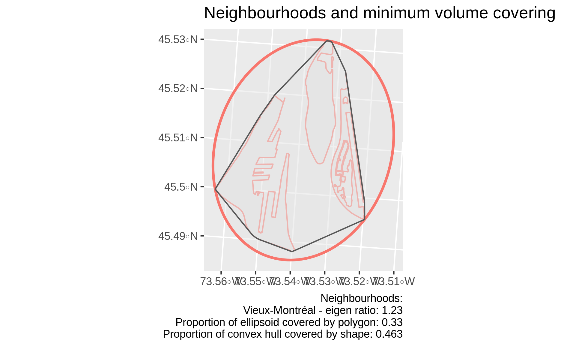
Neighbourhood with relatively symmetric MVE, but highly non-convex shape

This is an artefact of the otherwise desired convexity of the optimization problem and the covering ellipsoid found. In fact, the eigenratio is an indicator of symmetry of the convex hull of \(S\).

It may be interesting to also consider metrics such as the area of the convex hull of a shape covered by the shape: \(area(S)/area(conv(S)) \in [0,1]\), which indicates convexity of \(S\). An almost perfectly convex neighbourhood is illustrated in the figure below:

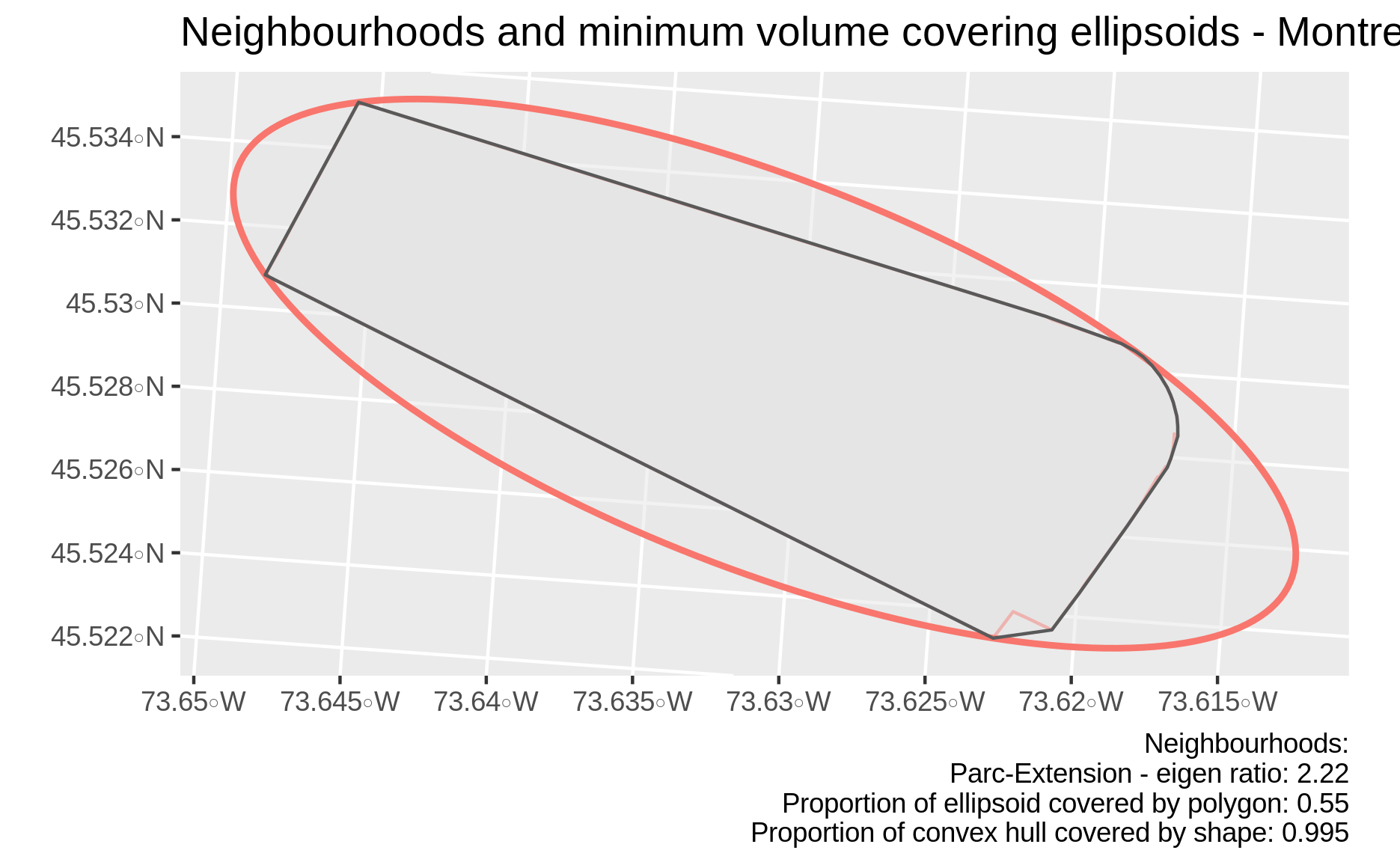
The most convex neighbourhood in Montreal is elongated